from IPython.display import Image
Image('../../Python_probability_statistics_machine_learning_2E.png',width=200)
%matplotlib inline

import matplotlib
matplotlib.rcParams['mathtext.fontset'] = 'cm'
matplotlib.rcParams['mathtext.rm'] = 'cm'
matplotlib.rcParams['mathtext.it'] = 'cm:italic'
matplotlib.rcParams['mathtext.bf'] = 'cm:bold'
import numpy as np
from matplotlib.pylab import subplots
Neural networks have a long history going back to the 1960s, but the recent availability of large-scale, high-quality data and new parallel computing infrastructures have reinvigorated neural networks in terms of size and complexity. This new reinvigoration, with many new and complex topologies, is called deep learning. There have been exciting developments in image and video processing, speech recognition, and automated video captioning based on deep learning systems. However, this is still a very active area of research. Fortunately, big companies with major investments in this area have made much of their research software open source (e.g., Tensorflow, PyTorch), with corresponding Python-bindings. To build up our understanding of neural networks, we begin with Rosenblatt's 1960 Perceptron.
Perceptron Learning
The perceptron is the primary ancestor of the most popular deep learning technologies (i.e., multilayer perceptron) and it is the best place to start as it will reveal the basic mechanics and themes of more complicated neural networks. The job of the perceptron is to create a linear classifier that can separate points in $\mathbb{R}^n$ between two classes. The basic idea is that given a set of associations:
where each $\mathbf{x}\in\mathbb{R}^{n-1}$ is augmented with a unit-entry to account for an offset term, and a set of weights $\mathbf{w}\in \mathbb{R}^n$, compute the following as an estimate of the label $y\in \lbrace -1,1 \rbrace$.
Concisely, this means that we want $\mathbf{w}$ such that
where $\mathbf{x}_i$ is in class $C_2$ if $\mathbf{x}_i^T\mathbf{w}>0$ and class $C_1$ otherwise. To determine these weights, we apply the following learning rule:
The output of the perceptron can be summarized as
The sign is the activation function of the perceptron. With this set up, we can write out the perceptron's output as the following:
import numpy as np
def yhat(x,w):
    return np.sign(np.dot(x,w))
Let us create some fake data to play with:
npts = 100
X=np.random.rand(npts,2)*6-3 # random scatter in 2-d plane
labels=np.ones(X.shape[0],dtype=np.int) # labels are 0 or 1
labels[(X[:,1]<X[:,0])]=-1
X = np.c_[X,np.ones(X.shape[0])] # augment with offset term
Note that we added a column of ones to account for the offset term. Certainly, by our construction, this problem is linearly separable, so let us see if the perceptron can find the boundary between the two classes. Let us start by initializing the weights,
winit = np.random.randn(3)
and then apply the learning rule,
w= winit
for i,j in zip(X,labels):
    w = w - (yhat(i,w)-j)*i
Note that we are taking a single ordered pass through the data. In practice, we would have randomly shuffled the input data to ensure that there is no incidental structure in the order of the data that would influence training. Now, let us examine the accuracy of the perceptron,
from sklearn.metrics import accuracy_score
print(accuracy_score(labels,[yhat(i,w) for i in X]))
We can re-run the training rule over the data to try to improve the accuracy. A pass through the data is called an epoch.
for i,j in zip(X,labels):
    w = w - (yhat(i,w)-j)*i

print(accuracy_score(labels,[yhat(i,w) for i in X]))
Note that our initial weight for this epoch is the last weight from the previous pass. It is common to randomly shuffle the data between epochs. More epochs will result in better accuracy in this case.
We can re-do this entire example with keras. First, we define the model,
from keras.models import Sequential
from keras.layers import Dense
from keras.optimizers import SGD
model = Sequential()
model.add(Dense(1, input_shape=(2,), activation='softsign'))
model.compile(SGD(), 'hinge')
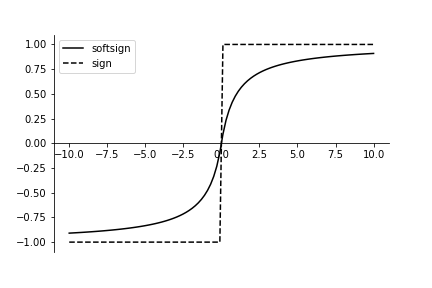
Note that we use the softsign activation instead of the sgn that
we used earlier because we need a differentiable activation function. Given
the form of the weight update in perceptron learning, it is equivalent to the
hinge loss function. Stochastic gradient descent (SGD) is chosen for
updating the weights. The softsign function is defined as the following:
We can pull it out from the tensorflow backend that keras uses as
in the following, plotted in Figure
import tensorflow as tf
x = tf.placeholder('float')
xi = np.linspace(-10,10,100)
with tf.Session() as s:
    y_=(s.run(tf.nn.softsign(x),feed_dict={x:xi}))
The softsign function is a smooth approximation to the sign function. This makes it easier to differentiate for backpropagation.
from matplotlib.pylab import subplots
fig,ax=subplots()
_=ax.plot(xi,y_,label='softsign',color='k')
_=ax.plot(xi,np.sign(xi),label='sign',linestyle='--',color='k')
_=ax.spines['top'].set_visible(False)
_=ax.spines['right'].set_visible(False)
_=ax.spines['bottom'].set_position(('data',0))
_=ax.legend()
fig.savefig('fig-machine_learning/deep_learning_002.png')
Next, all we have to do is fit the model on data,
h=model.fit(X[:,:2], labels, epochs=300, verbose=0)
The h variable is the history that contains the internal
metrics and parameters involved in the fit training phase. We can extract the
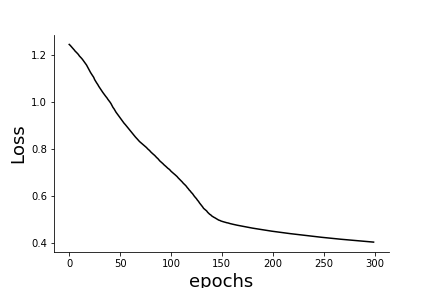
trajectory of the loss function from this history and draw the loss in
Figure.
fig,ax=subplots()
_=ax.plot(h.history['loss'],'k-')
_=ax.set_ylabel('Loss',fontsize=18)
_=ax.set_xlabel('epochs',fontsize=18)
_=ax.spines['top'].set_visible(False)
_=ax.spines['right'].set_visible(False)
fig.savefig('fig-machine_learning/deep_learning_003.png')
Trajectory of the loss function.
Multi-Layer Perceptron
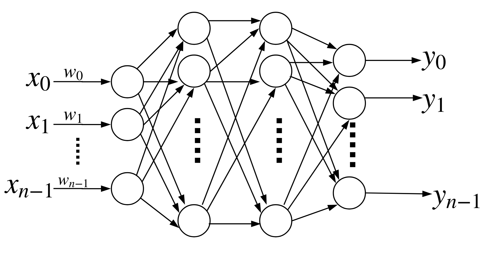
The Multi-Layer Perceptron (MLP) generalizes the perceptron by stacking them as fully connected individual layers. The basic topology is shown in Figure. In the previous section we saw that the basic perceptron could generate a linear boundary for data that is linearly separable. The MLP can create more complex nonlinear boundaries. Let us examine the moons dataset from scikit-learn,
The basic multi-layer perceptron has a single hidden layer between input and output. Each of the arrows has a multiplicative weight associated with it.
from sklearn.datasets import make_moons
X, y = make_moons(n_samples=1000, noise=0.1, random_state=1234)
The purpose of the noise term is to make data for each of the
categories harder to disambiguate. These data are shown in Figure
fig,ax=subplots()
_=ax.plot(X[y==0,0],X[y==0,1],'o',color='b',alpha=0.3)
_=ax.plot(X[y==1,0],X[y==1,1],'s',color='r',alpha=0.3)
_=ax.spines['top'].set_visible(False)
_=ax.spines['right'].set_visible(False)
fig.savefig('fig-machine_learning/deep_learning_004.png')
Data from make_moons.
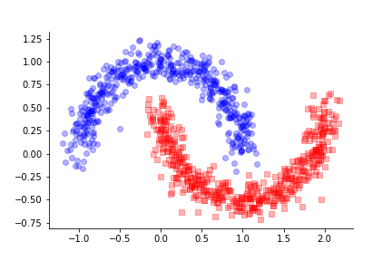
The challenge for the MLP is to derive a nonlinear boundary between these two
classes. We contruct our MLP using keras,
from keras.optimizers import Adam
model = Sequential()
model.add(Dense(4,input_shape=(2,),activation='sigmoid'))
model.add(Dense(2,activation='sigmoid'))
model.add(Dense(1,activation='sigmoid'))
model.compile(Adam(lr=0.05), 'binary_crossentropy')
This MLP has three layers. The input layer has four units and the
next layer has two units and the output layer has one unit to distinguish
between the two available classes. Instead of plain stochastic gradient
descent, we use the more advanced Adam optimizer. A quick
summary of the model elements and parameters comes
from the model.summary() method,
model.summary()
As usual, we split the input data into train and test sets,
from sklearn.model_selection import train_test_split
X_train,X_test,y_train,y_test=train_test_split(X,y,
                                               test_size=0.3,
                                               random_state=1234)
Thus, we reserve 30 percent of the data for testing. Next, we train the MLP,
h=model.fit(X_train, y_train, epochs=100, verbose=0)
To compute the accuracy metric using the test set, we need to compute the model prediction on the this set.
y_train_ = model.predict_classes(X_train,verbose=0)
y_test_ = model.predict_classes(X_test,verbose=0)
print(accuracy_score(y_train,y_train_))
print(accuracy_score(y_test,y_test_))
To visualize the so-derived boundary between these two classes, we
use the contourf function from matplotlib which generates a filled contour
plot shown in Figure.
xmin, ymin = X.min(axis=0)
xmax, ymax = X.max(axis=0)
xticks = np.linspace(xmin-0.1, xmax+0.1, 150)
yticks = np.linspace(ymin-0.1, ymax+0.1, 150)
xg,yg = np.meshgrid(xticks, yticks)
cg = model.predict(np.c_[xg.ravel(), yg.ravel()]).reshape(xg.shape)
fig,ax=subplots()
_=ax.plot(X[y==0,0],X[y==0,1],'o',color='b',alpha=0.3)
_=ax.plot(X[y==1,0],X[y==1,1],'s',color='r',alpha=0.3)
_=ax.contourf(xg,yg, cg, cmap='bwr', alpha=0.2)
fig.savefig('fig-machine_learning/deep_learning_005.png')
The derived boundary separates the two classes.

Instead of computing the accuracy separately, we can assign it as a
metric for keras to track by supplying it on the compile step, as in the
following,
model.compile(Adam(lr=0.05),
              'binary_crossentropy',
              metrics=['accuracy'])
Then, we can train again,
h=model.fit(X_train, y_train, epochs=100, verbose=0)
Now, we can evaluate the model on the test data,
loss,acc=model.evaluate(X_test,y_test,verbose=0)
print(acc)
where loss is the loss function and acc is the corresponding
accuracy. The documentation has other metrics that can be specified during the
compile step.
Backpropagation
We have seen that the MLP can generate complicated nonlinear boundaries for classification problems. The key algorithm underpinning MLP is backpropagation. The idea is that when we stack layers into the MLP, we are applying function composition, which basically means we take the output of one function and then feed it into the input of another.
For example, for the simple perceptron, we have $g(\mathbf{x}) = \mathbf{w}^T \mathbf{x}$ and $f(x) = \sgn(x)$. They key property of this composition is that derivatives use the chain rule from calculus.
Notice this has turned the differentiation operation into a multiplication operation. Explaining backpropagation in general is a notational nightmare, so let us see if we can get the main idea from a specific example. Consider the following two layer MLP with one input and one output.
There is only one input ($x_1$). The output of the first layer is
where $f$ is the sigmoid function and $b_1$ is the bias term. The output of the second layer is
To keep it simple, let us suppose that the loss function for this MLP is the squared error,
where $y$ is the target label. Backpropagation has two phases. The forward phase computes the MLP loss function given the values of the inputs and corresponding weights. The backward phase applies the incremental weight updates to each weight based on the forward phase. To implement gradient descent, we have to calculate the derivative of the loss function with respect to each of the weights.
The first term is the following,
The second term is the following,
Note that by property of the sigmoid function, we have $f'(x) = (1-f(x))f(x)$. The third term is the following,
Thus, the update for $w_2$ is the following,
The corresponding analysis fo $b_2$ gives the following,
Let's keep going backwards to $w_1$,
The first new term is the following,
and then the next two terms,
This makes the update for $w_1$,
To understand why this is called backpropagation, we can define
This makes the weight update for $w_2$,
This means that the weight update for $w_2$ is proportional to the output of the prior layer ($z_1$) and a factor that accounts steepness of the activation function. Likewise, the weight update for $w_1$ can be written as the following,
where
Note that this weight update is proportional to the input (prior layer's output) just as the weight update for $w_2$ was proportional to the prior layer output $z_1$. Also, the $\delta$ factors propagate recursively backwards to the input layer. These characteristics permit efficient numerical implementations for large networks because the subsequent computations are based on prior calculations. This also means that each individual unit's calculations are localized upon the output of the prior layer. This helps segregate the individual processing behavior of each unit within each layer.
Functional Deep Learning
Keras has an alternative API that makes it possible to
understand the performance of neural networks using the composition of
functions ideas we discussed. The key objects for this functional
interpretation are the Input object and the Model object.
from keras.layers import Input
from keras.models import Model
import keras.backend as K
We can re-create the data from our earlier classification example
from sklearn.datasets import make_moons
X, y = make_moons(n_samples=1000, noise=0.1, random_state=1234)
The first step is contruct a placeholder for the input using
the Input object,
inputs = Input(shape=(2,))
Next, we can stack the Dense layers as before but now tie their
inputs to the previous layer's outputs by calling Dense as a function.
l1=Dense(3,input_shape=(2,),activation='sigmoid')(inputs)
l2=Dense(2,input_shape=(3,),activation='sigmoid')(l1)
outputs=Dense(1,input_shape=(3,),activation='sigmoid')(l1)
This means that $\texttt{output}=(\ell_2 \circ \ell_1 )(\texttt{input})$
where $\ell_1$ and $\ell_2$ are the middle layers. With that established, we
collect the individual pieces in the the Model object and then fit and
train as usual.
model = Model(inputs=inputs,outputs=outputs)
model.compile(Adam(lr=0.05),
              'binary_crossentropy',
              metrics=['accuracy'])
h=model.fit(X_train, y_train, epochs=500, verbose=0)
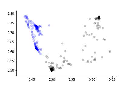
This gives the same result as before. The advantage of the functional perspective is that now we can think of the individual layers as mappings between multi-dimensional $\mathbb{R}^n$ spaces. For example, $\ell_1: \mathbb{R}^2 \mapsto \mathbb{R}^3$ and $\ell_2: \mathbb{R}^3 \mapsto \mathbb{R}^2$. Now, we can investigate the performance of the network from the inputs just up until the final mapping to $\mathbb{R}$ at the output by defining the functional mapping $(\ell_2 \circ \ell_1)(\texttt{inputs}): \mathbb{R}^2\mapsto \mathbb{R}^2$, as shown in Figure.
To get this result, we have to define a keras function using the inputs.
l2_function = K.function([inputs], [l2])
# functional mapping just before output layer
l2o=l2_function([X_train])
the l2o list contains the output of the l2 layer that
is shown in Figure.
l2_function = K.function([inputs], [l2])
# functional mapping just before output layer
l2o=l2_function([X_train])[0]

fig,ax=subplots()
_=ax.scatter(l2o[:,0],l2o[:,1],c=[ 'b' if i else 'k' for i in y_train],alpha=0.2)
_=ax.spines['top'].set_visible(False)
_=ax.spines['right'].set_visible(False)
fig.savefig('fig-machine_learning/deep_learning_006.png')
The embedded representation of the input just before the final output that shows the internal divergence of the two target classes.
Introduction to Tensorflow
Tensorflow is the leading deep learning framework. It is written in $\verb!C++!$ with Python bindings. Although we will primarily use the brilliant Keras abstraction layer to compose our neural networks with Tensorflow providing the backed computing, it is helpful to see how Tensorflow itself works and how to interact with it, especially for later debugging. To get started, import Tensorflow using the recommended convention.
import tensorflow as tf
Tensorflow is graph-based. We have to assemble a computational graph. To get started, let's define some constants,
# declare constants
a = tf.constant(2)
b = tf.constant(3)
The context manager (i.e., the with statement) is the recommended
way to create a session variable, which is a realization of the computational
graph that is composed of operations and tensor data objects. In this
context, a tensor is another word for a multidimensional matrix.
# default graph using the context manager
with tf.Session() as sess:
    print('a= ',a.eval())
    print('b= ',b.eval())
    print("a+b",sess.run(a+b))
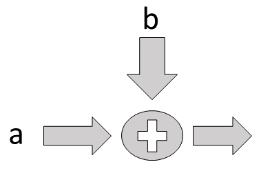
Thus, we can do some basic arithmetic on the declared variables. We can abstract the graph using placeholders. For example, to implement the computational graph shown in Figure, we can define the following,
Flow diagram for adder.
a = tf.placeholder(tf.int16)
b = tf.placeholder(tf.int16)
Next, we define the addition operation in the graph,
# declare operation
adder = tf.add(a,b)
Then, we compose and execute the graph using the context manager,
# default graph using context manager
with tf.Session() as sess:
    print (sess.run(adder, feed_dict={a: 2, b: 3}))
This works with matrices also, with few changes
import numpy as np
a = tf.placeholder('float',[3,5])
b = tf.placeholder('float',[3,5])
adder = tf.add(a,b)
with tf.Session() as sess:
   b_ = np.arange(15).reshape((3,5))
   print(sess.run(adder,feed_dict={a:np.ones((3,5)),
                                   b:b_}))
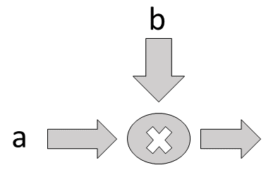
Matrix operations like multiplication are also implemented,
Flow diagram for multiplier
# the None dimension leaves it variable
b = tf.placeholder('float',[5,None])
multiplier = tf.matmul(a,b)
with tf.Session() as sess:
   b_ = np.arange(20).reshape((5,4))
   print(sess.run(multiplier,feed_dict={a:np.ones((3,5)),
                                        b:b_}))
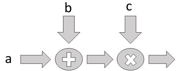
The individual computational graphs can be stacked as shown in Figure.
Flow diagram for adder and multiplier.
b = tf.placeholder('float',[3,5])
c = tf.placeholder('float',[5,None])
adder = tf.add(a,b)
multiplier = tf.matmul(adder,c)
with tf.Session() as sess:
   b_ = np.arange(15).reshape((3,-1))
   c_ = np.arange(20).reshape((5,4))
   print(sess.run(multiplier,feed_dict={a:np.ones((3,5)),
                                        b:b_,
                                        c:c_}))
Optimizers
To compute the parameters of complicated neural networks, a wide variety of optimization algorithms are also implemented in Tensorflow. Consider the classic least-squares problem: Find $\mathbf{x}$ that minimizes
First, we have to define a variable that we want the optimizer to solve for,
x = tf.Variable(tf.zeros((3,1)))
Next, we create sample matrices $\mathbf{A}$ and $\mathbf{b}$,
A = tf.constant([6,6,4,
                 3,4,0,
                 7,2,2,
                 0,2,1,
                 1,6,3],'float',shape=(5,3))
b = tf.constant([1,2,3,4,5],'float',shape=(5,1))
In neural network terminology, the output of the model ($\mathbf{A}\mathbf{x}$) is called the activation,
activation = tf.matmul(A,x)
The job of the optimizer is to minimize the squared distance between
the activation and the $\mathbf{b}$ vector. Tensorflow implements primitives
like reduce_sum to compute the square difference as a cost variable.
cost = tf.reduce_sum(tf.pow(activation-b,2))
With all that defined, we can construct the specific Tensorflow optimizer we want,
learning_rate = 0.001
optimizer=tf.train.GradientDescentOptimizer(learning_rate).minimize(cost)
The learning_rate is an embedded parameter for the
GradientDescentOptimizer gradient descent algorithm. Next, we
have to initialize all the variables,
init=tf.global_variables_initializer()
and create the session, without the context manager, just to show that the context manager is not a requirement,
sess = tf.Session()
sess.run(init)
costs=[]
for i in range(500):
   costs.append(sess.run(cost))
   sess.run(optimizer)
Note that we have to iterate over the optimizer to get it to
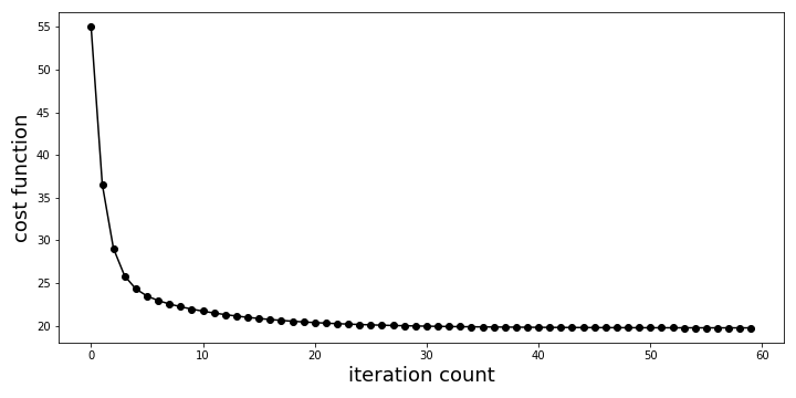
step-wise work through the gradient descent algorithm. As an illustration, we
can plot the change in the cost function as it iterates,
from matplotlib.pylab import subplots
fig,ax=subplots()
fig.set_size_inches((10,5))
_=ax.plot(costs[:60],'ok-',label='cost')
_=ax.set_xlabel('iteration count',fontsize=18)
_=ax.set_ylabel('cost function',fontsize=18)
_=fig.tight_layout()
fig.savefig('fig-machine_learning/LS_cost.png')
Iterative costs as gradient descent algorithm computes solution. Note that we are showing only a slice of all the values computed.
The final answer after all the iterations is the following,
print (x.eval(session=sess))
Because this is a classic problem, we know how to solve it analytically as in the following,
# least squares solution
A_=np.matrix(A.eval(session=sess))
print (np.linalg.inv(A_.T*A_)*(A_.T)*b.eval(session=sess))
which is pretty close to what we found by iterating.
Logistic Regression with Tensorflow
As an example, let us revisit the logistic regression problem using Tensorflow.
import numpy as np
from matplotlib.pylab import subplots
v = 0.9
@np.vectorize
def gen_y(x):
    if x<5: return np.random.choice([0,1],p=[v,1-v])
    else:   return np.random.choice([0,1],p=[1-v,v])

xi = np.sort(np.random.rand(500)*10)
yi = gen_y(xi)
from sklearn.linear_model import LogisticRegression
lr = LogisticRegression()
_=lr.fit(np.c_[xi],yi)
The simplest multi-layer perceptron has a single hidden layer. Given the training set $\lbrace \mathbf{x}_i,y_i \rbrace$ The input vector $\mathbf{x}_i$ is component-wise multiplied by the weight vector, $\mathbf{w}$ and then fed into the non-linear sigmoidal function. The output of the sigmoidal function is then compared to the training output, $y_i$, corresponding to the weight vector, to form the error. The key step after error-formation is the back-propagation step. This applies the chain-rule from calculus to transmit the differential error back to the weight vector.
Let's see if we can reproduce the logistic regression solution shown in Figure using Tensorflow. The first step is to import the Tensorflow module,
import tensorflow as tf
We need to reformat the training set slightly,
yi[yi==0]=-1 # use 1/-1 mapping
Then, we create the computational graph by creating variables and placeholders for the individual terms,
w = tf.Variable([0.1])
b = tf.Variable([0.1])
# the training set items fill these
x = tf.placeholder("float", [None])
y = tf.placeholder("float", [None])
The output of the neural network is sometimes called the activation,
activation = tf.exp(w*x + b)/(1+tf.exp(w*x + b))
The optimization problem is to reduce the following objective function, which includes the one-dimensional regularization term $w^2$,
# objective
obj=tf.reduce_sum(tf.log(1+tf.exp(-y*(b+w*x))))+tf.pow(w,2)
Given the objective function, we
choose the GradientDescentOptimizer as the optimization
algorithm with the embedded learning rate,
optimizer = tf.train.GradientDescentOptimizer(0.001/5.).minimize(obj)
Now, we are just about ready to start the session. But, first we need to initialize all the variables,
init=tf.global_variables_initializer()
We'll use an interactive session for convenience and then step through the optimization algorithm in the following loop,
s = tf.InteractiveSession()
s.run(init)
for i in range(1000):
   s.run(optimizer,feed_dict={x:xi,y:yi})
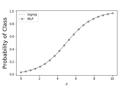
The result of this is shown in Figure which says that logistic regression and this simple single-layer perceptron both come up with the same answer.
fig,ax=subplots()
t = np.linspace(0,10,20)
_=ax.plot(t,lr.predict_proba(np.c_[t])[:,1],label='logreg',linestyle='--',color='k',alpha=0.3)
_=ax.plot(t,s.run(activation,feed_dict={x:t}),'-ko',label='MLP',alpha=0.3)
_=ax.legend(loc=0)
_=ax.set_xlabel('$x$',fontsize=16)
_=ax.set_ylabel('Probability of Class',fontsize=18)
fig.savefig('fig-machine_learning/deep_learning_001.png')
This shows the result from logistic regression as compared to the corresponding result from simple single-layer perceptron.
Understanding Gradient Descent
Consider a smooth function $f$ over $\mathbb{R}^n$ suppose we want to find the minimum value of $f(\mathbf{x})$ over this domain, as in the following,
The idea with gradient descent is to choose an initial point $\mathbf{x}^{(0)}\in \mathbb{R}^n$
where $\alpha$ is the step size (learning rate). The intuition here is that $\nabla f$ is the direction of increase and so that moving in the opposite direction scaled by $\alpha$ moves towards a lower function value. This approach turns out to be very fast for well-conditioned, strongly convex $f$ but in general there are practical issues.
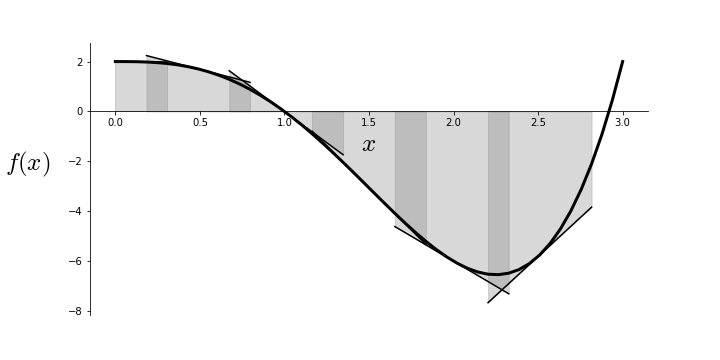
Figure shows the function $f(x) = 2 - 3 x^3 + x^4$ and its first-order Taylor series approximation at a selected points along the curve for a given width parameter. That is, the Taylor approximation approximates the function at a specific point with a corresponding interval around that point for which the approximation is assumed valid. The size of this width is determined by the $\alpha$ step parameter. Crucially, the quality of the approximation varies along the curve. In particular, there are sections where two nearby approximations overlap given the width, as indicated by the dark shaded regions. This is key because gradient descent works by using such first-order approximations to estimate the next step in the minimization. That is, the gradient descent algorithm never actually sees $f(x)$, but rather only the given first-order approximant. It judges the direction of the next iterative step by sliding down the slope of the approximant to the edge of a region (determined by $\alpha$) and then using that next point for the next calculated approximant. As shown by the shaded regions, it is possible that the algorithm will overshoot the minimum because the step size ($\alpha$) is too large. This can cause oscillations as shown in Figure.
import matplotlib
matplotlib.rcParams['mathtext.fontset'] = 'cm'
matplotlib.rcParams['mathtext.rm'] = 'cm'
matplotlib.rcParams['mathtext.it'] = 'cm:italic'
matplotlib.rcParams['mathtext.bf'] = 'cm:bold'
import numpy as np
from matplotlib.pylab import subplots
xi=np.linspace(0,3,50)

def get_chunk(x_0=1,delta=0.1,n=2):
    '''
    n := order of approximation
    '''
    x_0 = float(x_0)
    delta = float(delta)
    return fx.series(x,x0=sm.var('x0'),n=n).removeO().subs(x0,x_0),(x_0-delta<=x)&(x<x_0+delta)

def get_pw(x0list,delta = 0.1):
    pw=sm.lambdify(x,sm.Piecewise(*[get_chunk(float(i),delta) for i in x0list]))
    x0 = np.array(x0list)
    edges = np.vstack([x0-delta,x0+delta]).T
    return pw,edges

import sympy as sm
x = sm.var('x')
fx = 2 - 3*x**3 + x**4
fxx = sm.lambdify(x,fx)
pw,edges = get_pw(np.arange(0,3,0.5),.5/2.)

fig,ax= subplots()
fig.set_size_inches((10,5))
funcs= [sm.lambdify(x,sm.Piecewise(get_chunk(i,0.35))) for i in edges.mean(axis=1)]

_=ax.plot(xi,fxx(xi),lw=3,color='k')
_=ax.set_ylabel(r'$f(x)$'+' '*10,fontsize=25,rotation=0)
_=ax.set_xlabel(r'$x$',fontsize=25,rotation=0)
_=ax.spines['top'].set_visible(False)
_=ax.spines['right'].set_visible(False)
_=ax.spines['bottom'].set_position(('data',0))

for i in funcs:
    _=ax.fill_between(xi,i(xi),color='gray',alpha=0.3)
    _=ax.plot(xi,i(xi),color='k')

fig.savefig('fig-machine_learning/gradient_descent_001.png')
The piecewise linear approximant to $f(x)$.
Let us consider the following Python implementation of gradient descent, using Sympy.
x = sm.var('x')
fx = 2 - 3*x**3 + x**4
df = fx.diff(x) # compute derivative
x0 =.1 # initial guess
xlist = [(x0,fx.subs(x,x0))]
alpha = 0.1 # step size
for i in range(20):
    x0 = x0 - alpha*df.subs(x,x0)
    xlist.append((x0,fx.subs(x,x0)))
xlist = np.array(xlist).astype(float)
fig,ax= subplots()
fig.set_size_inches((8,5))
_=ax.plot(xlist[:,0],'-ok')
_=ax.set_xticks(range(0,21,2))
_=ax.set_xlabel('iteration ($k$)',fontsize=18)
_=ax.set_ylabel('$x_k$',fontsize=25)
_=ax.spines['top'].set_visible(False)
_=ax.spines['right'].set_visible(False)
fig.savefig('fig-machine_learning/gradient_descent_002.png')
Figure shows the sequential steps. Note that the algorithm oscillates at the end because the step size is too large. Practically speaking, it is not possible to know the optimal step size for general functions without strong assumptions on $f(x)$.
The step size may cause oscillations.
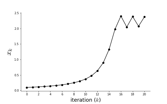
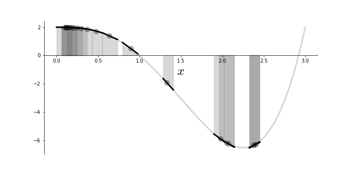
Figure shows how the algorithm moves along the function as well as the approximant ($\hat{f}(x)$) that the algorithm sees along the way. Note that initial steps are crowded around the initial point because the corresponding gradient is small there. Towards the middle, the algorithm makes a big jump because the gradient is steep, before finally oscillating towards the end. Sections of the underlying function that are relatively flat can cause the algorithm to converge very slowly. Furthermore, if there are multiple local minima, then the algorithm cannot guarantee finding the global minimum.
fig,ax= subplots()
fig.set_size_inches((10,5))
funcs= [sm.lambdify(x,sm.Piecewise(get_chunk(i,0.1))) for i in xlist[:,0]]
_=ax.plot(xlist[:,0],xlist[:,1],marker='o',ls='',markersize=10,alpha=.3,color='k',label=r'$f(x_k)$')
_=ax.plot(xi,fxx(xi),lw=3,color='lightgray',label='$f(x)$')
_=ax.set_xlabel(r'$x$',fontsize=25,rotation=0)
_=ax.spines['top'].set_visible(False)
_=ax.spines['right'].set_visible(False)
_=ax.spines['bottom'].set_position(('data',0))

for i in funcs:
    _=ax.fill_between(xi,i(xi),color='gray',alpha=0.3)
    _=ax.plot(xi,i(xi),color='k',lw=3,label=r'$\hat{f}(x)$')

fig.savefig('fig-machine_learning/gradient_descent_003.png')
Gradient descent produces a sequence of approximants.
As we have seen, the step size is key to both performance and convergence. Indeed, a step size that is too big can cause divergence and one that is too small can take a very long time to converge.
Newton's Method
Consider the following second-order Taylor series expansion
where $ \mathbf{H(x)} := \nabla^2 f(\mathbf{x})$ is the Hessian matrix of second derivatives. The $(i,j)^{th}$ entry of this matrix is the following:
We can use basic matrix calculus to find the minimum by computing:
Solving this for $\mathbf{x}$ gives the following:
Thus, after renaming some terms, the descent algorithm works by the following update equation:
There are a number of practical problems with this update equation. First, it requires computing the Hessian matrix at every step. For a significant problem, this means managing a potentially very large matrix. For example, given 1000 dimensions the corresponding Hessian has $1000 \times 1000$ elements. Some other issues are that the Hessian may not be numerically stable enough to invert, the functional form of the partial derivatives may have to be separately approximated, and the initial guess has to be in a region where the convexity of the function matches the derived assumption. Otherwise, just based on these equations, the algorithm will converge on the local maximum and not the local minimum. Consider a slight change of the previous code to implement Newton's method:
x0 =2. # init guess is near to solution
xlist = [(x0,fx.subs(x,x0))]
df2 = fx.diff(x,2) # 2nd derivative

for i in range(5):
    x0 = x0 - df.subs(x,x0)/df2.subs(x,x0)
    xlist.append((x0,fx.subs(x,x0)))

xlist = np.array(xlist).astype(float)
print (xlist)
Note that it took very few iterations to get to the minimum (as compared to our prior method), but if the initial guess is too far away from the actual minimum, the algorithm may not find the local minimum at all and instead find the local maximum. Naturally, there are many extensions to this method to account for these effects, but the main thrust of this section is to illustrate how higher-order derivatives (when available) in a computationally feasible context can greatly accelerate convergence of descent algorithms.
Managing Step Size
The problem of determining a good step size (learning rate) can be approached with an exact line search. That is, along the ray that extends along $\mathbf{x}+ q \nabla f(x)$, find
In words, this means that given a direction from a point $\mathbf{x}$ along the direction $\nabla f(\mathbf{x})$, find the minimum for this one-dimensional problem. Thus, the minimization procedure alternates at each iteration between moving to a new $\mathbf{x}$ position in $\mathbb{R}^n$ and finding a new step size by solving the one-dimensional minimization.
While this is conceptually clean, the problem is that solving the one-dimensional line-search at every step means evaluating the objective function $f(\mathbf{x})$ at many points along the one-dimensional slice. This can be very time consuming for an objective function that is computationally expensive to evaluate. With Newton's method, we have seen that higher-order derivatives can accelerate convergence and we can apply those ideas to the one-dimensional line search, as with the backtracking algorithm.
Fix parameters $\beta\in [0,1)$ an $\alpha>0$.
If $f(x-\alpha\nabla f(x))> f(x)- \alpha \Vert \nabla f(x) \Vert_2^2$ then reduce $\alpha\rightarrow \beta \alpha$. Otherwise, do the usual gradient descent update: $x^{(k+1)}= x^{(k)}-\alpha\nabla f(x^{(k)})$.
To gain some intuition about how this works, return to our second-order Taylor series expansion of the function $f$ about $\mathbf{x}_0$,
We have already discussed the numerical issues with the Hessian term, so one approach is to simply replace that term with an $n\times n$ identity matrix $\mathbf{I}$ to obtain the following:
This is our more tractable surrogate function. But what is the relationship between this surrogate and what we are actually trying to minimize? The key difference is that the curvature information that is contained in the Hessian term has now been reduced to a single $1/\alpha$ factor. Intuitively, this means that local complicated curvature of $f$ about a given point $\mathbf{x}_0$ has been replaced with a uniform bowl-shaped structure, the steepness of which is determined by scaling $1/\alpha$. Given a specific $\alpha$, we already know how to step directly to the minimum of $h_{\alpha}(\mathbf{x})$; namely, using the following gradient descent update equation:
That is the immediate solution to the surrogate problem, but it does not directly supply the next iteration for the function we really want: $f$. Let us suppose that our minimization of the surrogate has taken us to a new point $\mathbf{x}^{(k)}$ that satisfies the following inequality,
or, more explicitly,
We can substitute the update equation into this and simplify as,
which ultimately boils down to the following,
The important observation here is that if we have not reached the minimum of $f$, then the last term is always positive and we have moved downwards,
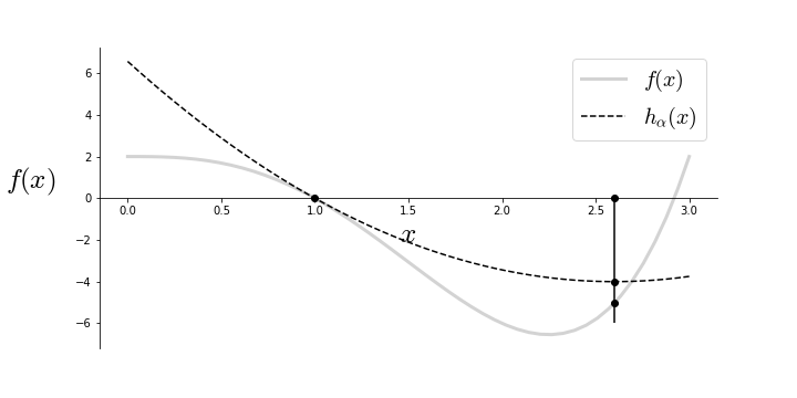
which is what we were after. Conversely, if the inequality in Equation (1) holds for some $\alpha>0$, then we know that $h_{\alpha}>f$. This is the key observation behind the backtracking algorithm. That is, we can test a sequence of values for $\alpha$ until we find one that satisfies Equation (1). For example, we can start with some initial $\alpha$ and then scale it up or down until the inequality is satisfied which means that we have found the correct step size and then can proceed with the descent step. This is what the backtracking algorithm is doing as shown in Figure. The dotted line is the $h_{\alpha}(x)$ and the gray line is $f(x)$. The algorithm hops to the quadratic minimum of the $h_{\alpha}(x)$ function which is close to the actual minimum of $f(x)$.
The basic implementation of backtracking is shown below:
x0 = 1
alpha = 0.5
xnew = x0 - alpha*df.subs(x,x0)
while fx.subs(x,xnew)>(fx.subs(x,x0)-(alpha/2.)*(fx.subs(x,x0))**2):
    alpha = alpha * 0.8
    xnew = x0 - alpha*df.subs(x,x0)

print (alpha,xnew)
fig,ax= subplots()
fig.set_size_inches((10,5))
_=ax.plot(xi,fxx(xi),lw=3,color='lightgray',label='$f(x)$')
ha = fx.subs(x,x0) + df.subs(x,x0)*(x-x0)+1/(alpha*2)*(x-x0)**2
haxx = sm.lambdify(x,ha)
_=ax.plot([1],[fxx(1)],'ok')

_=ax.plot(xi,haxx(xi),'--k',label=r'$h_{\alpha}(x)$')
_=ax.plot([xnew],[fxx(xnew)],'ok')
_=ax.plot([xnew],[haxx(xnew)],'ok')
_=ax.plot([xnew],[0],'ok')

_=ax.vlines(xnew,-6,0)
_=ax.set_xlabel(r'$x$',fontsize=25,rotation=0)
_=ax.spines['top'].set_visible(False)
_=ax.spines['right'].set_visible(False)
_=ax.spines['bottom'].set_position(('data',0))
_=ax.set_ylabel(r'$f(x)$'+' '*10,fontsize=25,rotation=0);

_=ax.legend(fontsize=20)

fig.savefig('fig-machine_learning/gradient_descent_004.png')
The approximation $h_{\alpha}(x)$ (dotted line) moves the next iteration from $x=1$ to the indicated point that is near the minimum of $f(x)$ by finding an appropriate step size ($\alpha$).
Stochastic Gradient Descent
A common variation on gradient descent is to alter how the weights are updated. Specifically, suppose we want to minimize an objective function of the following form:
where $i$ indexes the $i^{th}$ data element for an error function. Equivalently, each summand is parameterized by a data element.
For the usual gradient descent algorithm, we would compute the incremental weights, component-wise as in the following
by summing over all of the data. The key idea for stochastic gradient descent is to not sum over all of the data but rather to update the weights for each randomized $i^{th}$ data element:
A compromise between batch and this jump-every-time stochastic gradient descent is mini-batch gradient descent in which a randomized subset ($\sigma_r, \vert\sigma_r\vert=M_b$) of the data is summed over at each step as in the following:
Each step update for the standard gradient descent algorithm processes $m$ data points for each of the $p$ dimensions, $\mathcal{O}(mp)$, whereas for stochastic gradient descent, we have $\mathcal{O}(p)$. Mini-batch gradient descent is somewhere in-between these estimates. For very large, high-dimensional data, the computational costs of gradient descent can become prohibitive thus favoring stochastic gradient descent. Outside of the computational advantages, stochastic gradient descent has other favorable attributes. For example, the noisy jumping around helps the algorithm avoid getting stalled in local minima and this helps the algorithm when the starting point is far away from the actual minimum. The obverse is that stochastic gradient descent can struggle to clinch the minimum when it is close to it. Another advantage is robustness to a minority of bad data elements. Because only random subsets of the data are actually used in the update, the few individual outlier data points (perhaps due to poor data integrity) do not necessarily contaminate every step update.
Momentum
The gradient descent algorithm can be considered as a particle moving along a high-dimensional landscape in search of a minimum. Using a physical analogy, we can add the concept of momentum to the particle's motion. Consider the position of the particle ($\mathbf{x}^{(k)}$) at any time $k$ under a net force proportional to $-\nabla J$. This setup induces an estimated velocity term for the particle motion proportional to $\eta (\mathbf{x}^{(k+1)} - \mathbf{x}^{(k)}) $. That is, the particle's velocity is estimated proportional to the difference in two successive positions. The simplest version of stochastic gradient descent update that incorporates this momentum is the following:
Momentum is particularly useful when gradient descent sloshes up and down a steep ravine in the error surface instead of pursuing the descending ravine directly to the local minimum. This oscillatory behavior can cause slow convergence. There are many extensions to this basic idea such as Nesterov momentum.
Advanced Stochastic Gradient Descent
Methods that aggregate histories of the step updates can provide superior performance to the basic stochastic gradient descent algorithm. For example, Adam (Adaptive Moment Estimator) implements an adaptive step-size for each parameter. It also keeps track of an exponentially decaying mean and variance of past gradients using the exponentially weighted moving average (EWMA). This smoothing technique computes the following recursion,
with $y_0=x_0$ as the initial condition. The $0<a<1$ factor controls
the amount of mixing between the previous moving average and the new data point
at $n$. For example, if $a=0.9$, the EWMA favors the new data $x_n$ over the
prior value $y_{n-1}$ ($1-a=0.1$) of the EWMA. This calculation is common in a
wide variety of timeseries applications (i.e., signal processing, quantitative
finance). The impulse response of the EWMA ($x=\delta_n$) is $(1-a)^n$. You can
think of this as the weighted window function that is applied to $x_n$. As
opposed to the standard moving average that considers a fixed window of data to
average over, this exponential window retains prior memory of the entire
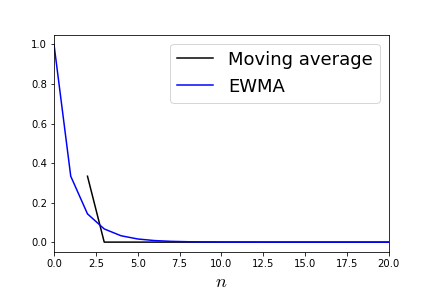
sequence, albeit weighted by powers of $(1-a)$. To see this, we can generate
the response to an impulse data series using pandas,
import pandas as pd
x = pd.Series([1]+[0]*20)
ma =x.rolling(window=3, center=False).mean()
ewma  = x.ewm(1).mean()
fig,ax= subplots()
_=ma.plot(ax=ax,label='Moving average',color='k')
_=ewma.plot(ax=ax,label='EWMA',color='b')
_=ax.legend(fontsize=18)
_=ax.set_xlabel('$n$',fontsize=18)
fig.savefig('fig-machine_learning/gradient_descent_005.png')
As shown by Figure, the single nonzero data point thereafter influences the EWMA whereas for the fixed-width moving window average, the effect terminates after the window passes. Note that mini-batch smoothes out data at each iteration by averaging over training data and EWMA smoothes out the descent motion across iterations of the algorithm.
The approxmation $h_{\alpha}(x)$ (dotted line) moves the next iteration from $x=1$ to the indicated point that is near the minimum of $f(x)$ by finding an appropriate step size ($\alpha$).
Advanced stochastic gradient descent algorithms are themselves an area of intense interest and development. Each method has its strengths and weaknesses pursuant to the data at hand (i.e., sparse vs. dense data) and there is no clear favorite appropriate to all circumstances. As a practical matter, some variants have parallel implementations that accelerate performance (i.e., Nui's Hogwild update scheme).
Python Example Using Sympy
Each of these methods will make more sense with some Python. We emphasize that this implementation is strictly expository and would not be suitable for a large-scale application. Let us reconsider the classification problem in the section on logistic regression with the target $y_i\in \lbrace 0,1 \rbrace$. The logistic regression seeks to minimize the cross-entropy:
with the corresponding gradient,
To get started let's create some sample data for logistic regression
import numpy as np
import sympy as sm
npts = 100
X=np.random.rand(npts,2)*6-3 # random scatter in 2-d plane
labels=np.ones(X.shape[0],dtype=np.int) # labels are 0 or 1
labels[(X[:,1]<X[:,0])]=0
This provides the data in the X Numpy array and the target labels
in the labels array. Next, we want to develop the objective function with Sympy,
x0,x1 = sm.symbols('x:2',real=True) # data placeholders
b0,b1 = sm.symbols('b:2',real=True) # parameters
bias = sm.symbols('bias',real=True) # bias term
y = sm.symbols('y',real=True) # label placeholders
summand = sm.log(1+sm.exp(x0*b0+x1*b1+bias))-y*(x0*b0+x1*b1+bias)
J = sum([summand.subs({x0:i,x1:j,y:y_i})
           for (i,j),y_i in zip(X,labels)])
We can use Sympy to compute the gradient as in the following:
from sympy.tensor.array import derive_by_array
grad = derive_by_array(summand,(b0,b1,bias))
Using the sm.latex function renders grad as the
following:
which matches our previous computation of the gradient. For standard gradient descent, the gradient is computed by summing over all of the data,
grads=np.array([grad.subs({x0:i,x1:j,y:y_i})
                    for (i,j),y_i in zip(X,labels)]).sum(axis=0)
Now, to implement gradient descent, we set up the following loop:
# convert expression into function
Jf = sm.lambdify((b0,b1,bias),J)
gradsf = sm.lambdify((b0,b1,bias),grads)
niter = 200
winit = np.random.randn(3)*20
alpha = 0.1 # learning rate (step-size)
WK = winit  # initialize
Jout=[] # container for output
for i in range(niter):
    WK = WK - alpha * np.array(gradsf(*WK))
    Jout.append(Jf(*WK))
For stochastic gradient descent, the above code changes to the following:
import random
sgdWK = winit  # initialize
Jout=[] # container for output
# don't sum along all data as before
grads=np.array([grad.subs({x0:i,x1:j,y:y_i})
                    for (i,j),y_i in zip(X,labels)])
for i in range(niter):
    gradsf = sm.lambdify((b0,b1,bias),random.choice(grads))
    sgdWK = sgdWK - alpha * np.array(gradsf(*sgdWK))
    Jout.append(Jf(*sgdWK))
The main difference here is that the gradient calculation no longer
sums across all of the input data (i.e., grads list) and is instead randomly
chosen by the random.choice function the above body of the loop. The
extension to batch gradient descent from this code just requires
averaging over a sub-selection of the data for the gradients in the
batch variable.
mbsgdWK = winit  # initialize
Jout=[] # container for output
mb = 10 # number of elements in batch
for i in range(niter):
    batch = np.vstack([random.choice(grads)
                          for i in range(mb)]).mean(axis=0)
    gradsf = sm.lambdify((b0,b1,bias),batch)
    mbsgdWK = mbsgdWK-alpha*np.array(gradsf(*mbsgdWK))
    Jout.append(Jf(*mbsgdWK))
It is straight-forward to incorporate momentum into this loop using a
Python deque, as in the following,
from collections import deque
momentum = deque([winit,winit],2)
mbsgdWK = winit  # initialize
Jout=[] # container for output
mb = 10 # number of elements in batch
for i in range(niter):
    batch=np.vstack([random.choice(grads)
                       for i in range(mb)]).mean(axis=0)
    gradsf=sm.lambdify((b0,b1,bias),batch)
    mbsgdWK=mbsgdWK-alpha*np.array(gradsf(*mbsgdWK))+0.5*(momentum[1]-momentum[0])
    Jout.append(Jf(*mbsgdWK))
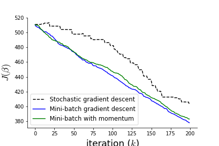
Figure shows the three variants of the gradient descent algorithm. Notice that the stochastic gradient descent algorithm is the most erratic, as it is characterized by taking a new direction for every randomly selected data element. Mini-batch gradient descent smoothes these out by averaging across multiple data elements. The momentum variant is somewhere in-between the to as the effect of the momentum term is not pronounced in this example.
Different variations of gradient descent.
Python Example Using Theano
The code shown makes each step of the gradient descent algorithms explicit
using Sympy, but this implementation is far too slow. The theano module
provides thoughtful and powerful high-level abstractions for algorithm
implementation that relies upon underlying C/C++ and GPU execution models. This
means that calculations that are prototyped with theano can be executed
downstream outside of the Python interpreter which makes them much faster. The
downside of this approach is that calculations can become much harder to
debug because of the multiple levels of abstraction. Nonetheless, theano is
a powerful tool for algorithm development and execution.
To get started we need some basics from theano.
import theano
import theano.tensor as T
from theano import function, shared
the next step is to define variables, which are essentially placeholders for values that will be computed downstream later. The next block defines two named variables as a double-sized float matrix and vector. Note that we did not have to specify the dimensions of each at this point.
x = T.dmatrix("x") # double matrix
y = T.dvector("y") # double vector
The parameters of our implementation of gradient descent come next, as the following:
w = shared(np.random.randn(2), name="w") # parameters to fit
b = shared(0.0, name="b") # bias term
variables that are shared are ones whose values can be set
separately via other computations or directly via the set_value() method.
These values can also be retrieved using the get_value() method. Now, we need
to define the probability of obtaining a 1 from the given data as p. The
cross-entropy function and the T.dot function are already present (along with
a wide range of other related functions) in theano. The conformability of
the constituent arguments is the responsibility of the user.
p=1/(1+T.exp(-T.dot(x,w)-b)) # probability of 1
error = T.nnet.binary_crossentropy(p,y)
loss = error.mean()
gw, gb = T.grad(loss, [w, b])
The error variable is TensorVariable type which has many
built-in methods such as mean. The so-derived loss function is therefore
also a TensorVariable. The last T.grad line is the best part of Theano because
it can compute these gradients automatically.
train = function(inputs=[x,y],
                 outputs=[error],
                 updates=((w, w - alpha * gw),
                          (b, b - alpha * gb)))
The last step is to set up training by defining the training function
in theano. The user will supply the previously defined and named input
variables (x and y) and theano will return the previously defined error
variable. Recall that the w and b variables were defined as shared
variables. This means that the function train can update their values between
calls using the update formula specified in the updates keyword variable. In
this case, the update is just plain gradient descent with the previously
defined alpha step-size variable.
We can execute the training plain using the train function in the following loop:
training_steps=1000
for i in range(training_steps):
    error = train(X, labels)
The train(X,labels) call is where the X and labels arrays we
defined earlier replace the placeholder variables. The update step refreshes
all of the shared variables at each iterative step. At the end of the
iteration, the so-computed parameters are in the w and b variables with
values available via get_value(). The implementation for stochastic gradient
descent requires just a little modification to this loop, as in the following:
for i in range(training_steps):
    idx = np.random.randint(0,X.shape[0])
    error = train([X[idx,:]], [labels[idx]])
where the idx variable selects a random data element from the set and
uses that for the update step at every iteration. Likewise, batch stochastic
gradient descent follows with the following modification,
batch_size = 50
indices = np.arange(X.shape[0])
for i in range(training_steps):
    idx = np.random.permutation(indices)[:batch_size]
    error = train(X[idx,:], labels[idx])

print (w.get_value())
print (b.get_value()) # bias term
Here, we set up an indices variable that is used for randomly
selecting subsets in the idx variable that are passed to the train
function. All of these implementations parallel the corresponding previous
implementations in Sympy, but these are many orders of magnitude faster due to
theano.
Image Processing Using Convolutional Neural Networks
import numpy as np
from matplotlib.pylab import subplots, cm
def text_grid(res,i,j,t,ax,**kwds):
    '''
    put text `t` on grid `i,j` position
    passing down `kwds` to `ax.text`
    '''
    assert isinstance(t,str)
    assert isinstance(res,np.ndarray)
    color = kwds.pop('color','r')
    ax.text(i-0.25,j+0.25,t,color=color,**kwds)

def text_grid_array(res,ax=None,fmt='%d',title=None,title_kw=dict(),**kwds):
    '''
    put values of `res` array as text on grid
    '''
    assert isinstance(res,np.ndarray)
    if ax is None:
        fig, ax = subplots()
    ax.imshow(res,cmap=cm.gray_r)
    ii,jj = np.where(res.T)
    for i,j in zip(ii,jj):
        text_grid(res,i,j,fmt%(res[j,i]),ax,**kwds)
    if title:
        ax.set_title(title,**title_kw)
    try:
        return fig
    except:
        pass

def draw_ndimage(c,m=4,n=5,figsize=[10,10]):
    t,mt,nt = c.shape
    assert m*n == t
    fig,axs=subplots(m,n,figsize=figsize)
    for ax,i in zip(axs.flatten(),c):
        text_grid_array(i,fontsize=6,fmt='%.1f',ax=ax)
        _= ax.tick_params(labelleft=False,left=False,labelbottom=False,bottom=False)
    return fig
In this section, we develop the Convolutional Neural Network (CNN) which is the
fundamental deep learning image processing application. We deconstruct every
layer of this network to develop insight into the purpose of the individual
operations. CNNs take image as inputs and images can be represented as
Numpy arrays, which makes them fast and easy to use with any of the scientific
Python tools. The individual entries of the Numpy array are the pixels and the
row/column dimensions are the height/width of the image respectively. The
array values are between 0 through 255 and correspond to the intensity of
the pixel at that location. Three-dimensional images have a third
third depth-dimension as the color channel (e.g., red, green,
blue). Two-dimensional image arrays are grayscale.
Programming Tip.
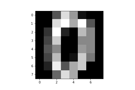
Matplotlib makes it easy to draw images using the underlying Numpy arrays. For
instance, we can draw Figure using the following
MNIST image from sklearn.datasets, which represents grayscale hand-drawn
digits (the number zero in this case).
from matplotlib.pylab import subplots, cm
from sklearn import datasets
mnist = datasets.load_digits()
fig, ax = subplots()
ax.imshow(mnist.images[0],
          interpolation='nearest',
          cmap=cm.gray)
fig.savefig('fig-machine_learning/image_processing_001.png')
The cmap keyword argument specifies the colormap as gray. The
interpolation keyword means that the resulting image from imshow does not
try to visually smooth out the data, which can be confusing when working at the
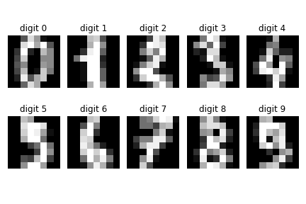
pixel level. The other hand drawn digits are shown below in Figure.
Image of a hand drawn number zero from the MNIST dataset.
fig, axs = subplots(2,5, constrained_layout=False)
fig.tight_layout()
for i,(ax,j) in enumerate(zip(axs.flatten(),mnist.images)):
   _=ax.imshow(j,interpolation='nearest',cmap=cm.gray)
   _=ax.set_title('digit %d'%(i))
   _=ax.spines['top'].set_visible(False)
   _=ax.spines['bottom'].set_visible(False)
   _=ax.spines['left'].set_visible(False)
   _=ax.spines['right'].set_visible(False)
   _=ax.spines['top'].axis.set_ticks_position('none')
   _=ax.spines['bottom'].axis.set_ticks_position('none')
   _=ax.spines['left'].axis.set_ticks_position('none')
   _=ax.spines['right'].axis.set_ticks_position('none')
   _=ax.xaxis.set_visible(False)
   _=ax.yaxis.set_visible(False)

fig.tight_layout()
fig.savefig('fig-machine_learning/image_processing_002.png')
Samples of the other hand drawn digits from MNIST.
Convolution
Convolution is an intensive calculation and it is the core of convolutional
neural networks. The purpose of convolution is to create alternative
representations of the input image that emphasize or demphasize certain
features represented by the kernel. The convolution operation consists of a
kernel and an input matrix. The convolution operation is a way of aligning
and comparing image data with the corresponding data in an image kernel. You
can think of an image kernel as a template for a canonical feature that the
convolution operation will uncover. To keep it simple suppose we have the
following 3x3 kernel matrix,
import numpy as np
kern = np.eye(3,dtype=np.int)
kern
Using this kernel, we want to find anything in an input image that looks like a diagonal line. Let's suppose we have the following input Numpy image
tmp = np.hstack([kern,kern*0])
x = np.vstack([tmp,tmp])
x
Note that this image is just the kernel stacked into a larger Numpy
array. We want to see if the convolution can pull out the kernel that is
embedded in the image. Of course, in a real application we would not know
whether or not the kernel is present in the image, but this example
helps us understand the convolution operation step-by-step. There is a
convolution function available in the scipy module.
from scipy.ndimage.filters import convolve
res = convolve(x,kern,mode='constant',cval=0)
res
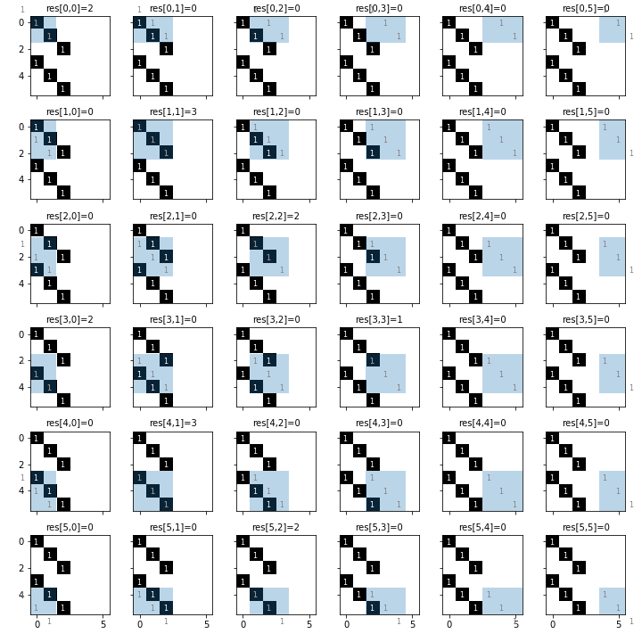
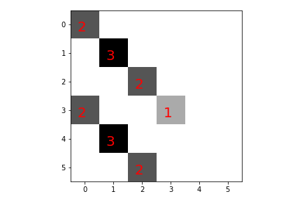
Each step of the convolution operation is represented in Figure. The kern matrix (light blue square) is
overlaid upon the x matrix and the element-wise product is computed and
summed. Thus, the 0,0 array output corresponds to this operation applied to
the top-left 3x3 slice of the input, which results in 3. The convolution
operation is sensitive to boundary conditions. For this example, we have chosen
mode=constant and cval=0 which means that the input image is bordered by
zeros when the kernel sweeps outside of the input image boundary. This is the
simplest option for managing the edge conditions and
scipy.ndimage.filters.convolve provides other practical alternatives. It also
common to normalize the output of the convolution operation by dividing by the
number of pixels in the kernel (i.e., 3 in this example). Another way to
think about the convolution operation is as a matched filter that peaks when it
finds a compatible sub-feature. The final output of the convolution operation
is shown in Figure. The values of the
individual pixels are shown in color. Notice where the maximum values of the
output image are located on the diagonals.
The convolution process that produces the res array. As shown in the sequence, the light blue kern array is slid around, overlaid, mutiplied, and summed upon the x array to generate the values of shown in the title. The output of the convolution is shown in [Figure](#fig:image_processing_004).
The res array output of the convolution is shown in [Figure](#fig:image_processing_003). The values (in red) shown are the individual outputs of the convolution operation. The grayscale indicates relative magnitude of the shown values (darker is greater).
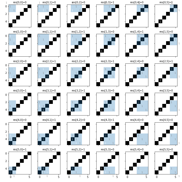
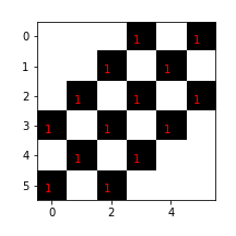
However, the convolution operation is not a perfect detector and results in nonzero values for other cases. For example, suppose the input image is a forward-slash diagonal line. The step-by-step convolution with the kernel is shown in Figure with corresponding output in Figure that looks nothing like the kernel or the input image.
The input array is a forward slash diagonal. This sequence shows the step-by-step convolution operation. The output of this convolution is shown in [Figure](#fig:image_processing_006).
The output of the convolution operation shown in [Figure](#fig:image_processing_005). Note that the output has nonzero elements where there is no match between the input image and the kernel.
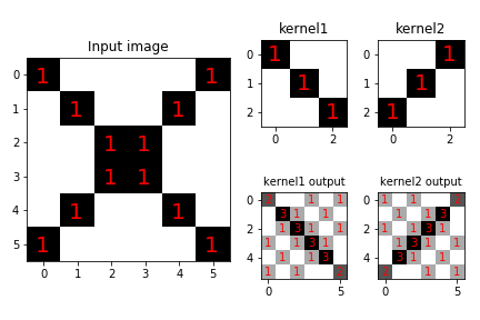
We can use multiple kernels to explore an input image. For example, suppose we have the input image shown on the left in Figure. The two kernels are shown in the upper row, with corresponding outputs on the bottom row. Each kernel is able to emphasize its particular feature but extraneous features appear in both outputs. We can have as many outputs as we have kernels but because each output image is as large as the input image, we need a way to reduce the size of this data.
Given two kernels (upper row) and the input image on the left, the output images are shown on the bottom row. Note that each kernel is able to emphasize its feature on the input composite image but other extraneous features appear in the outputs.
Maximum Pooling
To reduce the size of the output images, we can apply maximum pooling to replace a tiled subset of the image with the maximum pixel value in that particular subset. The following Python code illustrates maximum pooling,
def max_pool(res,width=2,height=2):
    m,n = res.shape
    xi = [slice(i,i+width) for i in range(0,m,width)]
    yi = [slice(i,i+height) for i in range(0,n,height)]
    out = np.zeros((len(xi),len(yi)),dtype=res.dtype)
    for ni,i in enumerate(xi):
        for nj,j in enumerate(yi):
            out[ni,nj]= res[i,j].max()
    return out
Programming Tip.
The slice object provides programmatic array slicing. For
example, x[0,3]=x[slice(0,3)]. This means you can
separate the slice from the array, which makes it easier to manage.
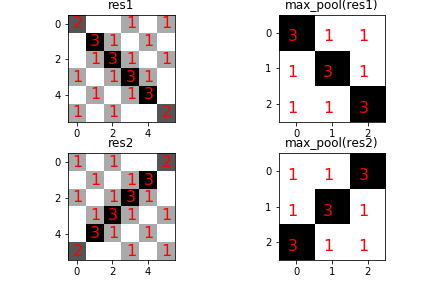
Pooling reduces the dimensionality of the output of the convolution
and makes stacking convolutions together computationally feasible. Figure shows the output of the max_pool function on
the indicated input images.
The max_pool function reduces the size of the output images (left column) to the images on the right column. Note that the pool size is 2x2 so that the resulting pooled images are half the size of the original images in each dimension.
Rectified Linear Activation
Rectified Linear Activation Units (ReLUs) are neural network units that implement the following activation function,
To use this activation properly, the kernels in the convolutional layer must be scaled to the $\lbrace -1,1 \rbrace$ range. We can implement our own rectified linear activation function using the following code,
def relu(x):
    'rectified linear activation function'
    out = np.zeros(x.shape,dtype=x.dtype)
    idx = x>=0
    out[idx]=x[idx]
    return out
Now that we understand the basic building blocks, let us investigate how the operations fit together. To create some training image data, we use the following function to create some random backwards and forwards slashed images as shown in Figure. As before, we have the scaled kernels shown in Figure. We are going to apply the convolution, max-pooling, and rectified linear activation function sequence step-by-step and observe the outputs at each step.
def gen_rand_slash(m=6,n=6,direction='back'):
    '''generate random forward/backslash images.
    Must have at least two pixels'''
    assert direction in ('back','forward')
    assert n>=2 and m>=2
    import numpy as np
    import random
    out = -np.ones((m,n),dtype=float)
    i = random.randint(2,min(m,n))
    j = random.randint(-i,max(m,n)-1)
    t = np.diag([1,]*i,j)
    if direction == 'forward':
        t = np.flipud(t)
    try:
        assert t.sum().sum()>=2
        out[np.where(t)]=1
        return out
    except:
        return gen_rand_slash(m=m,n=n,direction=direction)

# create slash-images training data with classification id 1 or 0
training=[(gen_rand_slash(),1) for i in range(10)] + \
         [(gen_rand_slash(direction='forward'),0) for i in range(10)]
fig,axs=subplots(4,5,figsize=[8,8])
for ax,i in zip(axs.flatten(),training):
    _=ax.imshow(i[0],cmap='gray_r')
    _=ax.set_title(f'category={i[1]}')
    _=ax.tick_params(labelleft=False,left=False,labelbottom=False,bottom=False)

fig.tight_layout()
fig.savefig('fig-machine_learning/image_processing_009.png')
The training data set for our convolutional neural network. The forward slash images are labelled category 0 and the backward slash images are category 1.

The two scaled feature kernels for the convolutional neural network.
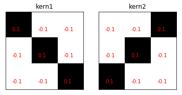
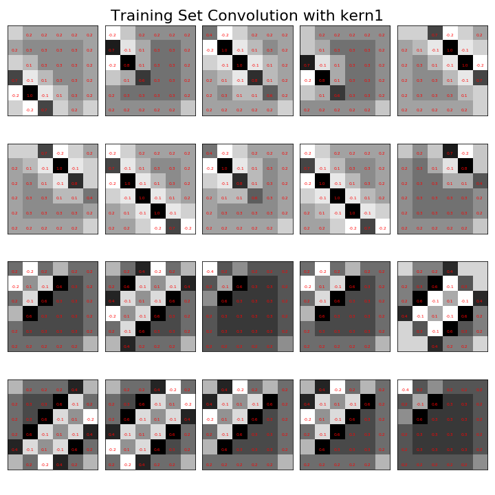
Figure shows the output of convolving the
training data in Figure with kern1, as shown on
the left panel of Figure. Note that
the following code defines each of these kernels,
kern1 = (np.eye(3,dtype=np.int)*2-1)/9. # scale
kern2 = np.flipud(kern1)
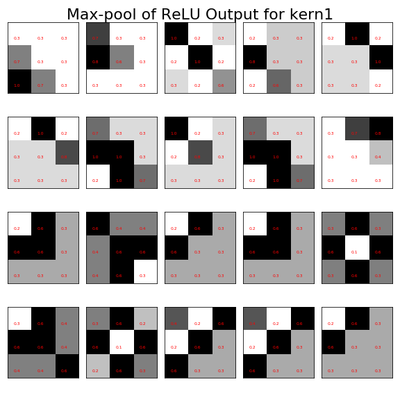
The next operation is the activation function for the rectified linear unit with output shown in Figure. Note that all of the negative terms have been replaced by zeros. The next step is the maximum pooling operation as shown in Figure. Notice that the number of total pixels in the training data has reduced from thirty-six per image to nine per image. With these processed images, we have the inputs we need for the final classification step.
fig,axs=subplots(4,5,figsize=[10,10])
for ax,(i,cat) in zip(axs.flatten(),training):
    res1=convolve(i,kern1,mode='constant',cval=0)
    _= text_grid_array(res1,fontsize=6,fmt='%.1f',ax=ax)
    _= ax.tick_params(labelleft=False,left=False,labelbottom=False,bottom=False)

_=fig.suptitle('Training Set Convolution with kern1',fontsize=22)
fig.tight_layout()
fig.savefig('fig-machine_learning/image_processing_011.png')
fig,axs=subplots(4,5,figsize=[10,10])

for ax,(i,cat) in zip(axs.flatten(),training):
    res1=convolve(i,kern1,mode='constant',cval=0)
    _=text_grid_array(relu(res1),fontsize=6,fmt='%.1f',ax=ax)
    _=ax.tick_params(labelleft=False,left=False,labelbottom=False,bottom=False)

_=fig.suptitle('ReLU of Convolution with kern1',fontsize=22)
fig.tight_layout()
fig.savefig('fig-machine_learning/image_processing_012.png')
fig,axs=subplots(4,5,figsize=[8,8])
for ax,(i,cat) in zip(axs.flatten(),training):
    res1=convolve(i,kern1,mode='constant',cval=0)
    tmp= max_pool(relu(res1))
    _=text_grid_array(tmp,fontsize=6,fmt='%.1f',ax=ax)
    _=ax.tick_params(labelleft=False,left=False,labelbottom=False,bottom=False)

_=fig.suptitle('Max-pool of ReLU Output for kern1',fontsize=22)
fig.tight_layout()
fig.savefig('fig-machine_learning/image_processing_013.png')
The output of convolving the training data in [Figure](#fig:image_processing_009) with kern1, as shown on the left panel of [Figure](#fig:image_processing_010).
The output of the rectified linear unit activation function with the input shown in [Figure](#fig:image_processing_011).

The output of maximum pooling operation with the input shown in [Figure](#fig:image_processing_012) for fixed image kernel kern1.
Convolutional Neural Network Using Keras
Now that we have experimented with the individual operations using our own Python code, we can construct the convolutional neural network using Keras. In particular, we use the Keras functional interface to define this neural network because that makes it easy to unpack the operations at the individual layers.
from keras import metrics
from keras.models import Model
from keras.layers.core import Dense, Activation, Flatten
from keras.layers import Input
from keras.layers.convolutional import Conv2D
from keras.layers.pooling import MaxPooling2D
from keras.optimizers import SGD
from keras import backend as K
from keras.utils import to_categorical
Note that the names of the modules are consistent with their
operations. We also need to tell Keras how to manage the input images,
K.set_image_data_format('channels_first') # image data format
inputs = Input(shape=(1,6,6)) # input data shape
Now we can build the individual convolutional layers. Note the specification of
the activations at each layer and placement of the inputs.`
clayer = Conv2D(2,(3,3),padding='same',
            input_shape=(1,6,6),name='conv',
            use_bias=False,
            trainable=False)(inputs)

relu_layer= Activation('relu')(clayer)
maxpooling = MaxPooling2D(pool_size=(2,2),
                          name='maxpool')(relu_layer)
flatten = Flatten()(maxpooling)
softmax_layer = Dense(2,
                      activation='softmax',
                      name='softmax')(flatten)
model = Model(inputs=inputs, outputs=softmax_layer)
# inject fixed kernels into convolutional layer
fixed_kernels = [np.dstack([kern1,kern2]).reshape(3,3,1,2)]
model.layers[1].set_weights(fixed_kernels)
Observe that the functional interface means that each layer is
explicitly a function of the previous one. Note that trainable=False for the
convolutional layer because we want to inject our fixed kernels into it at the
end. The flatten layer reshapes the data so that the entire processed image
at the point is fed into the softmax_layer, whose output is proportional to
the probability that the image belongs to either class. The set_weights()
function is where we inject our fixed kernels. These are not going to be
updated by the optimization algorithm because of the prior trainable=False
option. With the topology of the neural network defined, we now have to choose
the optimization algorithm and pack all of this configuration into the model
with the compile step.
lr = 0.01 # learning rate
sgd = SGD(lr=lr, decay=1e-6, momentum=0.9, nesterov=True)
model.compile(loss='categorical_crossentropy',
              optimizer=sgd,
              metrics=['accuracy',
                       metrics.categorical_crossentropy])
The metrics specification means that we want to training process to
keep track of those named items. Next, we generate some training data using our
gen_rand_slash function with the associated class of each image (1 or 0).
Most of this code is just shaping the tensors for Keras. The final
model.fit() step is where the internal weights of the neural network are
adjusted according to the given inputs.
# generate some training data
ntrain = len(training)
t=np.dstack([training[i][0].T
               for i in range(ntrain)]).T.reshape(ntrain,1,6,6)
y_binary=to_categorical(np.hstack([np.ones(ntrain//2),
                                   np.zeros(ntrain//2)]))
# fit the configured model
h=model.fit(t,y_binary,epochs=500,verbose=0)
With that completed, we can investigate the functional mapping of each layer
with K.function. The following creates a mapping between the input layer and
the convolutional layer,
convFunction = K.function([inputs],[clayer])
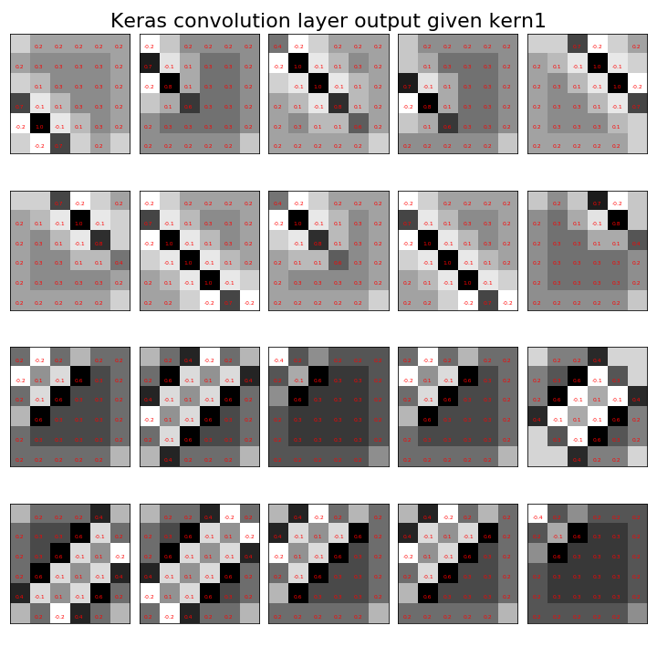
Now, we can feed the training data into this function as see the output of just the convolutional layer, which is shown,
fig=draw_ndimage(convFunction([t])[0][:,0,:,:],4,5)
_=fig.suptitle('Keras convolution layer output given kern1',fontsize=22);
fig.tight_layout()
fig.savefig('fig-machine_learning/image_processing_015.png')
fig=draw_ndimage(convFunction([t])[0][:,1,:,:],4,5)
_=fig.suptitle('Keras convolution layer output given kern2',fontsize=22);
fig.tight_layout()
fig.savefig('fig-machine_learning/image_processing_016.png')
Compare this to [Figure](#fig:image_processing_011). This shows our hand-tooled convolution is the same as that implemented by Keras.
We can do this again for the pooling layer by creating another Keras function,
maxPoolingFunction = K.function([inputs],[maxpooling])
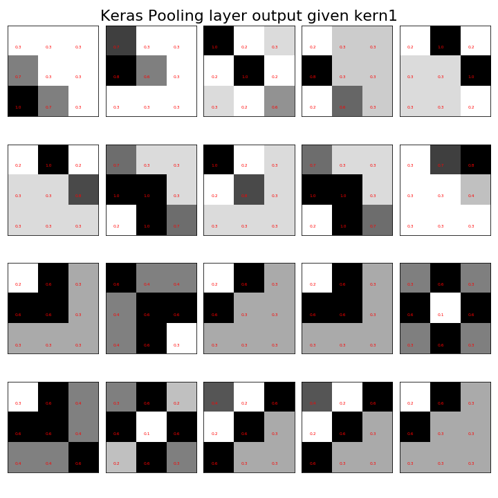
whose output is shown in Figure. We can examine the
final output of this network using the predict function,
fixed_kernels = model.predict(t)
fixed_kernels
and we can see the weights given to each of the classes. Taking the maximum of these across the columns gives the following,
np.argmax(fixed_kernels,axis=1)
which means that our convolutional neural network with the fixed kernels
did well predicting the classes of each of our input images. Recall that our model
configuration prevented our fixed kernels from updating in the training process. Thus, the
main work of model training was changing the weights of the final output layer. We can
re-do this exercise by removing this constraint and see how the network performs if
it is able to adaptively re-weight the kernel terms as part of training by changing the trainable
keyword argument and then re-build and train the model, as shown next.
clayer = Conv2D(2,(3,3),padding='same',
            input_shape=(1,6,6),name='conv',
            use_bias=False)(inputs)

relu_layer= Activation('relu')(clayer)
maxpooling = MaxPooling2D(pool_size=(2,2),
                          name='maxpool')(relu_layer)
flatten = Flatten()(maxpooling)
softmax_layer = Dense(2,
                      activation='softmax',
                      name='softmax')(flatten)
model = Model(inputs=inputs, outputs=softmax_layer)
model.compile(loss='categorical_crossentropy',
              optimizer=sgd)
h=model.fit(t,y_binary,epochs=500,verbose=0)
new_kernels = model.predict(t)
new_kernels
with corresponding max output,
np.argmax(new_kernels,axis=1)
fig=draw_ndimage(maxPoolingFunction([t])[0][:,0,:,:],4,5)
_=fig.suptitle('Keras Pooling layer output given kern1',fontsize=22);
fig.tight_layout()
fig.savefig('fig-machine_learning/image_processing_017.png')
Output of max-pooling layer for fixed kernel kern1. Compare this to [Figure](#fig:image_processing_013). This shows our hand-tooled implemention is equivalent to that by Keras.
fig,axs=subplots(1,2,sharey=True,sharex=True)
text_grid_array(model.layers[1].get_weights()[0][:,:,0,0],fmt='%.1f',title='Updated kern1',ax=axs[0])
text_grid_array(model.layers[1].get_weights()[0][:,:,0,1],fmt='%.1f',title='Updated kern2',ax=axs[1])
for ax in axs:
    ax.tick_params(labelleft=False,left=False,labelbottom=False,bottom=False)

fig.savefig('fig-machine_learning/image_processing_018.png')
Kernels updated during the training process. Compare to [Figure](#fig:image_processing_010).
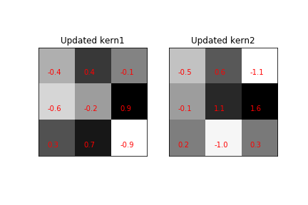
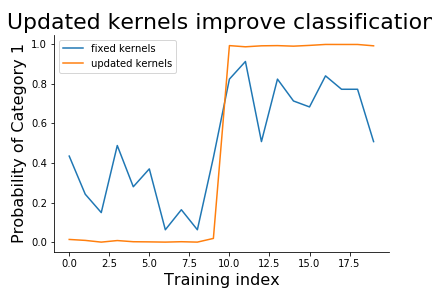
The newly updated kernels are shown in Figure. Note how different these are from the original fixed kernels. We can see the change in the respective predictions in Figure. Thus, the benefit of updating the kernels in the training process is to improve the accuracy overall, but at the cost of interpretability of the kernels themselves. Nonetheless, it is seldom the case that the kernels are known ahead of time, as in our artificial example here, so in practice, there may be nothing to really interpet anyway. Nonetheless, for other problems where there is a target feature in the data for which good a-priori exemplars exist that could serve a kernels, then priming these kernels early in training may help to tune into those target features, especially if they are rare in the training data.
fig,ax=subplots()
_=ax.plot(fixed_kernels[:,0],label='fixed kernels')
_=ax.plot(new_kernels[:,0],label='updated kernels')
_=ax.set_xlabel('Training index',fontsize=16)
_=ax.set_ylabel('Probability of Category 1',fontsize=16)
_=ax.spines['top'].set_visible(False)
_=ax.spines['right'].set_visible(False)
_=ax.legend()
_=ax.set_title('Updated kernels improve classification',fontsize=22)
fig.savefig('fig-machine_learning/image_processing_019.png')
Recall that the second half of the training set was classified as category 1. The updated kernels provide a wider margin for classification than our fixed kernels, even though the ultimate performance is very similar between them.
