from IPython.display import Image
Image('../../Python_probability_statistics_machine_learning_2E.png',width=200)

Logistic regression is one example of a wider class of Generalized Linear Models (GLMs). These GLMs have the following three key features

A target $Y$ variable distributed according to one of the exponential family of distributions (e.g., Normal, binomial, Poisson)
An equation that links the expected value of $Y$ with a linear combination of the observed variables (i.e., $\left\{ x_1,x_2,\ldots,x_n \right\}$).
A smooth invertible link function $g(x)$ such that $g(\mathbb{E}(Y)) = \sum_k \beta_k x_k$

Exponential Family¶

Here is the one-parameter exponential family,

$$ f(y;\lambda) = e^{\lambda y - \gamma(\lambda)} $$

The natural parameter is $\lambda$ and $y$ is the sufficient statistic. For example, for logistic regression, we have $\gamma(\lambda)=-\log(1+e^{\lambda})$ and $\lambda=\log{\frac{p}{1-p}}$.

An important property of this exponential family is that

$$ \begin{equation} \mathbb{E}_{\lambda}(y) = \frac{d\gamma(\lambda)}{d\lambda}=\gamma'(\lambda) \end{equation} \label{eq:dgamma} \tag{1} $$

To see this, we compute the following,

$$ \begin{align*} 1 &= \int f(y;\lambda) dy = \int e^{\lambda y - \gamma(\lambda)} dy \\ 0 &= \int \frac{df(y;\lambda)}{d\lambda} dy =\int e^{\lambda y-\gamma (\lambda)} \left(y-\gamma'(\lambda)\right) dy \\ \int y e^{\lambda y-\gamma (\lambda )} dy &= \mathbb{E}_{\lambda}(y)=\gamma'(\lambda ) \end{align*} $$

Using the same technique, we also have,

$$ \mathbb{V}_{\lambda}(Y) = \gamma''(\lambda) $$

which explains the usefulness of this generalized notation for the exponential family.

Deviance¶

The scaled Kullback-Leibler divergence is called the deviance as defined below,

$$ D(f_1,f_2) = 2 \int f_1(y) \log{\frac{f_1(y)}{f_2(y)}}dy $$

Hoeffding's Lemma.

Using our exponential family notation, we can write out the deviance as the following,

$$ \begin{align*} \frac{1}{2} D(f(y;\lambda_1), f(y;\lambda_2)) & = \int f(y;\lambda_1)\log \frac{f(y;\lambda_1)}{f(y;\lambda_2)} dy \\ & = \int f(y;\lambda_1) ((\lambda_1-\lambda_2) y -(\gamma(\lambda_1)-\gamma(\lambda_2))) dy \\ & = \mathbb{E}_{\lambda_1} [ (\lambda_1-\lambda_2) y -(\gamma(\lambda_1)-\gamma(\lambda_2)) ] \\ & = (\lambda_1-\lambda_2) \mathbb{E}_{\lambda_1}(y) -(\gamma(\lambda_1)-\gamma(\lambda_2)) \\ & = (\lambda_1-\lambda_2) \mu_1 -(\gamma(\lambda_1)-\gamma(\lambda_2)) \end{align*} $$

where $\mu_1:=\mathbb{E}_{\lambda_1}(y)$. For the maximum likelihood estimate $\hat{\lambda}_1$, we have $\mu_1=y$. Plugging this into the above equation gives the following,

$$ \begin{align*} \frac{1}{2} D(f(y;\hat{\lambda}_1),f(y;\lambda_2))&=(\hat{\lambda}_1-\lambda_2) y -(\gamma(\hat{\lambda}_1)-\gamma(\lambda_2)) \\ &= \log{f(y;\hat{\lambda}_1)} - \log{f(y;\lambda_2)} \\ &= \log\frac{f(y;\hat{\lambda}_1)}{f(y;\lambda_2)} \end{align*} $$

Taking the negative exponential of both sides gives,

$$ f(y;\lambda_2) = f(y;\hat{\lambda}_1) e^{-\frac{1}{2} D(f(y;\hat{\lambda}_1),f(y;\lambda_2)) } $$

Because $D$ is always non-negative, the likelihood is maximized when the the deviance is zero. In particular, for the scalar case, it means that $y$ itself is the best maximum likelihood estimate for the mean. Also, $f(y;\hat{\lambda}_1)$ is called the saturated model. We write Hoeffding's Lemma as the following,

$$ \begin{equation} f(y;\mu) = f(y;y)e^{-\frac{1}{2} D(f(y;y),f(y;\mu))} \end{equation} \label{eq:lemma} \tag{2} $$

to emphasize that $f(y;y)$ is the likelihood function when the mean is replaced by the sample itself and $f(y;\mu)$ is the likelihood function when the mean is replaced by $\mu$.

Vectorizing Equation (2) using mutual independence gives the following,

$$ f(\mathbf{y};\boldsymbol{\mu}) = e^{-\sum_i D(y_i,\mu_i)} \prod f(y_i;y_i) $$

The idea now is to minimize the deviance by deriving,

$$ \boldsymbol{\mu}(\boldsymbol{\beta}) = g^{-1}(\mathbf{M}^T\boldsymbol{\beta}) $$

This means the the MLE $\hat{\boldsymbol{\beta}}$ is the best $p\times 1$ vector $\boldsymbol{\beta}$ that minimizes the total deviance where $g$ is the link function and $\mathbf{M}$ is the $p\times n$ structure matrix. This is the key step with GLM estimation because it reduces the number of parameters from $n$ to $p$. The structure matrix is where the associated $x_i$ data enters into the problem. Thus, GLM maximum likelihood fitting minimizes the total deviance like plain linear regression minimizes the sum of squares.

With the following,

$$ \boldsymbol{\lambda} = \mathbf{M}^T \boldsymbol{\beta} $$

with $2\times n$ dimensional $\mathbf{M}$. The corresponding joint density function is the following,

$$ f(\mathbf{y};\beta)=e^{\boldsymbol{\beta}^T\boldsymbol{\xi}-\psi(\boldsymbol{\beta})} f_0(\mathbf{y}) $$

where

$$ \boldsymbol{\xi} = \mathbf{M} \mathbf{y} $$

and

$$ \psi(\boldsymbol{\beta}) = \sum \gamma(\mathbf{m}_i^T \boldsymbol{\beta}) $$

where now the sufficient statistic is $\boldsymbol{\xi}$ and the parameter vector is $\boldsymbol{\beta}$, which fits into our exponential family format, and $\mathbf{m}_i$ is the $i^{th}$ column of $\mathbf{M}$.

Given this joint density, we can compute the log likelihood as the following,

$$ \ell = \boldsymbol{\beta}^T\boldsymbol{\xi}-\psi(\boldsymbol{\beta}) $$

To maximize this likelihood, we take the derivative of this with respect to $\boldsymbol{\beta}$ to obtain the following,

$$ \frac{d\ell}{d\boldsymbol{\beta}}=\mathbf{M}\mathbf{y}-\mathbf{M}\boldsymbol{\mu}(\mathbf{M}^T\boldsymbol{\beta}) $$

since $\gamma'(\mathbf{m}_i^T \boldsymbol{\beta}) = \mathbf{m}_i^T \mu_i(\boldsymbol{\beta})$ and (c.f. Equation (1)), $\gamma' = \mu_{\lambda}$. Setting this derivative equal to zero gives the conditions for the maximum likelihood solution,

$$ \begin{equation} \mathbf{M}(\mathbf{y}- \boldsymbol{\mu}(\mathbf{M}^T\boldsymbol{\beta})) = \mathbf{0} \end{equation} \label{eq:conditions} \tag{3} $$

where $\boldsymbol{\mu}$ is the element-wise inverse of the link function. This leads us to exactly the same place we started: trying to regress $\mathbf{y}$ against $\boldsymbol{\mu}(\mathbf{M}^T\boldsymbol{\beta})$.

Example¶

The structure matrix $\mathbf{M}$ is where the $x_i$ data associated with the corresponding $y_i$ enters the problem. If we choose

$$ \mathbf{M}^T = [\mathbf{1}, \mathbf{x}] $$

where $\mathbf{1}$ is an $n$-length vector and

$$ \boldsymbol{\beta} = [\beta_0, \beta_1]^T $$

with $\mu(x) = 1/(1+e^{-x})$, we have the original logistic regression problem.

Generally, $\boldsymbol{\mu}(\boldsymbol{\beta})$ is a nonlinear function and thus we regress against our transformed variable $\mathbf{z}$

$$ \mathbf{z} = \mathbf{M}^T\boldsymbol{\beta} + \diag(g'(\boldsymbol{\mu}))(\mathbf{y}-\boldsymbol{\mu}(\mathbf{M}^T\boldsymbol{\beta})) $$

This fits the format of the Gauss Markov (see ch:stats:sec:gauss) problem and has the

following solution,

$$ \begin{equation} \hat{\boldsymbol{\beta}}=(\mathbf{M} \mathbf{R}_z^{-1}\mathbf{M}^T)^{-1}\mathbf{M} \mathbf{R}_z^{-1}\mathbf{z} \end{equation} \label{eq:bhat} \tag{4} $$

where

$$ \mathbf{R}_z:=\mathbb{V}(\mathbf{z})=\diag(g'(\boldsymbol{\mu}))^2\mathbf{R}=\mathbf{v}(\mu)\diag(g'(\boldsymbol{\mu}))^2\mathbf{I} $$

where $g$ is the link function and $\mathbf{v}$ is the variance function on the designated distribution of the $y_i$. Thus, $\hat{\boldsymbol{\beta}}$ has the following covariance matrix,

$$ \mathbb{V}(\hat{\boldsymbol{\beta}}) = (\mathbf{M}\mathbf{R}_z^{-1}\mathbf{M}^T)^{-1} $$

These results allow inferences about the estimated parameters $\hat{\boldsymbol{\beta}}$. We can easily write Equation (4) as an iteration as follow,

$$ \hat{\boldsymbol{\beta}}_{k+1}=(\mathbf{M} \mathbf{R}_{z_k}^{-1}\mathbf{M}^T)^{-1}\mathbf{M} \mathbf{R}_{z_k}^{-1}\mathbf{z}_k $$

Example¶

Consider the data shown in Figure. Note that the variance of the data increases for each $x$ and the data increases as a power of $x$ along $x$. This makes this data a good candidate for a Poisson GLM with $g(\mu) = \log(\mu)$.

%matplotlib inline

from scipy.stats.distributions import poisson
import statsmodels.api as sm
from matplotlib.pylab import subplots
import numpy as np

def gen_data(n,ns=10):
    param = n**2
    return poisson(param).rvs(ns)

fig,ax=subplots()
xi = []
yi = []
for i in [2,3,4,5,6]:
    xi.append([i]*10)
    yi.append(gen_data(i))
    _=ax.plot(xi[-1],yi[-1],'ko',alpha=.3)

_=ax.axis(xmin=1,xmax=7)
xi = np.array(xi)
yi = np.array(yi)
x = xi.flatten()
y = yi.flatten()
_=ax.set_xlabel('x');
fig.savefig('fig-machine_learning/glm_003.png')

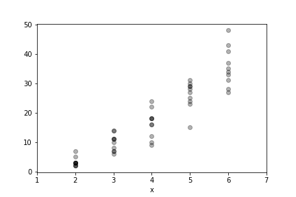
Some data for Poisson example.

We can use our iterative matrix-based approach. The following code initializes the iteration.

M   = np.c_[x*0+1,x].T
gi  = np.exp             # inverse g link function
bk  = np.array([.9,0.5]) # initial point
muk = gi(M.T @ bk).flatten() 
Rz  = np.diag(1/muk)
zk  = M.T @ bk + Rz @ (y-muk)

and this next block establishes the main iteration

while abs(sum(M @ (y-muk))) > .01: # orthogonality condition as threshold
   Rzi = np.linalg.inv(Rz)
   bk = (np.linalg.inv(M @ Rzi @ M.T)) @ M @ Rzi @ zk
   muk = gi(M.T @ bk).flatten()
   Rz =np.diag(1/muk)
   zk = M.T @ bk + Rz @ (y-muk)

with corresponding final $\boldsymbol{\beta}$ computed as the following,

print(bk)

[0.72758176 0.48763741]

with corresponding estimated $\mathbb{V}(\hat{\boldsymbol{\beta}})$ as

print(np.linalg.inv(M @ Rzi @ M.T))

[[ 0.01850392 -0.0035621 ]
 [-0.0035621   0.00072885]]

The orthogonality condition Equation (3) is the following,

print(M @ (y-muk))

[-4.90472131e-05 -2.62970365e-04]

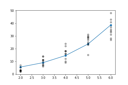
For comparison, the statsmodels module provides the Poisson GLM object. Note that the reported standard error is the square root of the diagonal elements of $\mathbb{V}(\hat{\boldsymbol{\beta}})$. A plot of the data and the fitted model is shown below in Figure (fig:glm_004).

pm=sm.GLM(y, sm.tools.add_constant(x), 
                        family=sm.families.Poisson())
pm_results=pm.fit()
pm_results.summary()

b0,b1=pm_results.params
fig,ax=subplots()
_=ax.plot(xi[:,0],np.exp(xi[:,0]*b1+b0),'-o');
_=ax.plot(xi,yi,'ok',alpha=.3);
fig.savefig('fig-machine_learning/glm_004.png')
_=ax.set_xlabel('x');

Fitted using the Poisson GLM.

Dep. Variable:	y	No. Observations:	50
Model:	GLM	Df Residuals:	48
Model Family:	Poisson	Df Model:	1
Link Function:	log	Scale:	1.0000
Method:	IRLS	Log-Likelihood:	-143.03
Date:	Tue, 27 Aug 2019	Deviance:	63.998
Time:	13:19:09	Pearson chi2:	62.0
No. Iterations:	5
Covariance Type:	nonrobust

	coef	std err	z	P>\|z\|	[0.025	0.975]
const	0.7276	0.136	5.348	0.000	0.461	0.994
x1	0.4876	0.027	18.060	0.000	0.435	0.541