from IPython.display import Image
Image('../../Python_probability_statistics_machine_learning_2E.png',width=200)
The features from a particular dataset that will ultimately prove important for machine learning can be difficult to know ahead of time. This is especially true for problems that do not have a strong physical underpinning. The row-dimension of the input matrix ($X$) for fitting data in Scikit-learn is the number of samples and the column dimension is the number of features. There may be a large number of column dimensions in this matrix, and the purpose of dimensionality reduction is to somehow reduce these to only those columns that are important for the machine learning task.
Fortunately, Scikit-learn provides some powerful tools to help uncover the most relevant features. Principal Component Analysis (PCA) consists of taking the input $X$ matrix and (1) subtracting the mean, (2) computing the covariance matrix, and (3) computing the eigenvalue decomposition of the covariance matrix. For example, if $X$ has more columns than is practicable for a particular learning method, then PCA can reduce the number of columns to a more manageable number. PCA is widely used in statistics and other areas beyond machine learning, so it is worth examining what it does in some detail. First, we need the decomposition module from Scikit-learn.
from sklearn import decomposition
import numpy as np
pca = decomposition.PCA()
Let's create some very simple data and apply PCA.
x = np.linspace(-1,1,30)
X = np.c_[x,x+1,x+2] # stack as columns
pca.fit(X)
print(pca.explained_variance_ratio_)
Programming Tip.
The np.c_ is a shorcut method for creating stacked column-wise arrays.
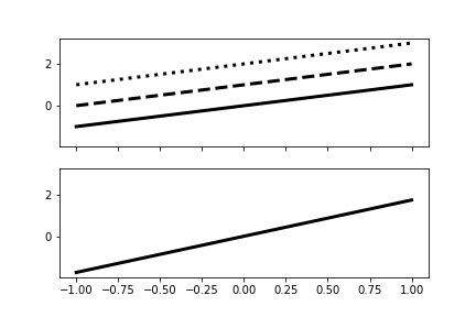
In this example, the columns are just constant offsets of the first
column. The explained variance ratio is the percentage of the variance
attributable to the transformed columns of X. You can think of this as the
information that is relatively concentrated in each column of the transformed
matrix X. Figure shows the graph of this dominant
transformed column in the bottom panel. Note that a constant offset in each of
the columns does not change its respective variance and thus, as far as PCA is
concerned, the three columns are identical from an information standpoint.
%matplotlib inline

from matplotlib.pylab import subplots
fig,axs = subplots(2,1,sharex=True,sharey=True)
ax = axs[0]
_=ax.plot(x,X[:,0],'-k',lw=3)
_=ax.plot(x,X[:,1],'--k',lw=3)
_=ax.plot(x,X[:,2],':k',lw=3)
ax=axs[1]
_=ax.plot(x,pca.fit_transform(X)[:,0],'-k',lw=3)
#ax.tick_params(labelsize='x-large')
fig.savefig('fig-machine_learning/pca_001.png')
The top panel shows the columns of the feature matrix and the bottom panel shows the dominant component that PCA has extracted.
To make this more interesting, let's change the slope of each of the columns as in the following,
X = np.c_[x,2*x+1,3*x+2,x] # change slopes of columns
pca.fit(X)
print(pca.explained_variance_ratio_)
However, changing the slope did not impact the explained variance ratio. Again, there is still only one dominant column. This means that PCA is invariant to both constant offsets and scale changes. This works for functions as well as simple lines,
x = np.linspace(-1,1,30)
X = np.c_[np.sin(2*np.pi*x),
          2*np.sin(2*np.pi*x)+1,
          3*np.sin(2*np.pi*x)+2]
pca.fit(X)
print(pca.explained_variance_ratio_)
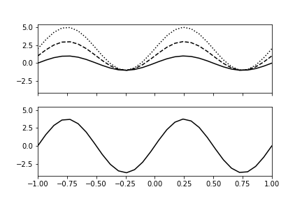
Once again, there is only one dominant column, which is shown in the bottom panel of Figure. The top panel shows the individual columns of the feature matrix. To sum up, PCA is able to identify and eliminate features that are merely linear transformations of existing features. This also works when there is additive noise in the features, although more samples are needed to separate the uncorrelated noise from between features.
The top panel shows the columns of the feature matrix and the bottom panel shows the dominant component that PCA has computed.
fig,axs = subplots(2,1,sharex=True,sharey=True)
ax = axs[0]
_=ax.plot(x,X[:,0],'-k')
_=ax.plot(x,X[:,1],'--k')
_=ax.plot(x,X[:,2],':k')
ax=axs[1]
_=ax.axis(xmin=-1,xmax=1)
_=ax.plot(x,pca.fit_transform(X)[:,0],'-k')
# ax.tick_params(labelsize='x-large')
fig.savefig('fig-machine_learning/pca_002.png')
fig,axs=subplots(1,2,sharey=True)
ax=axs[0]
_=ax.axis(xmin=-2,xmax=12)
x1 = np.arange(0, 10, .01/1.2)
x2 = x1+ np.random.normal(loc=0, scale=1, size=len(x1))
X = np.c_[(x1, x2)]
good = (x1>5) | (x2>5)
bad = ~good
_=ax.plot(x1[good],x2[good],'o',alpha=.3,color='gray')
_=ax.plot(x1[bad],x2[bad],'ok',alpha=.3)
_=ax.set_title("original data space")
_=ax.set_xlabel("x")
_=ax.set_ylabel("y")

_=pca.fit(X)
Xx=pca.fit_transform(X)
ax=axs[1]
# ax.set_aspect(1/1.6)
_=ax.plot(Xx[good,0],Xx[good,1]*0,'o',alpha=.3,color='gray')
_=ax.plot(Xx[bad,0],Xx[bad,1]*0,'ok',alpha=.3)
_=ax.set_title("PCA-reduced data space")
_=ax.set_xlabel(r"$\hat{x}$")
_=ax.set_ylabel(r"$\hat{y}$")
fig.savefig('fig-machine_learning/pca_003.png')
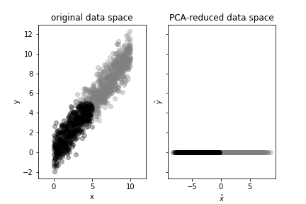
To see how PCA can simplify machine learning tasks, consider Figure wherein the two classes are separated along the diagonal.
After PCA, the transformed data lie along a single axis where the two classes
can be split using a one-dimensional interval, which greatly simplifies the
classification task. The class identities are preserved under PCA because the
principal component is along the same direction that the classes are separated.
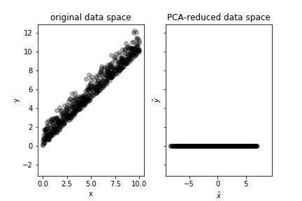
On the other hand, if the classes are separated along the direction
orthogonal to the principal component, then the two classes become mixed
under PCA and the classification task becomes much harder. Note that in both
cases, the explained_variance_ratio_ is the same because the explained
variance ratio does not account for class membership.
The left panel shows the original two-dimensional data space of two easily distinguishable classes and the right panel shows the reduced the data space transformed using PCA. Because the two classes are separated along the principal component discovered by PCA, the classes are preserved under the transformation.
fig,axs=subplots(1,2,sharey=True)
ax=axs[0]
x1 = np.arange(0, 10, .01/1.2)
x2 = x1+np.random.normal(loc=0, scale=1, size=len(x1))
X = np.c_[(x1, x2)]
good = x1>x2
bad = ~good
_=ax.plot(x1[good],x2[good],'ow',alpha=.3)
_=ax.plot(x1[bad],x2[bad],'ok',alpha=.3)
_=ax.set_title("original data space")
_=ax.set_xlabel("x")
_=ax.set_ylabel("y")

_=pca.fit(X)
Xx=pca.fit_transform(X)
ax=axs[1]
_=ax.plot(Xx[good,0],Xx[good,1]*0,'ow',alpha=.3)
_=ax.plot(Xx[bad,0],Xx[bad,1]*0,'ok',alpha=.3)
_=ax.set_title("PCA-reduced data space")
_=ax.set_xlabel(r"$\hat{x}$")
_=ax.set_ylabel(r"$\hat{y}$")

fig.savefig('fig-machine_learning/pca_004.png')
As compared with [Figure](#fig:pca_003), the two classes differ along the coordinate direction that is orthogonal to the principal component. As a result, the two classes are no longer distinguishable after transformation.
PCA works by decomposing the covariance matrix of the data using the Singular Value Decomposition (SVD). This decomposition exists for all matrices and returns the following factorization for an arbitrary matrix $\mathbf{A}$,
Because of the symmetry of the covariance matrix, $\mathbf{U} = \mathbf{V}$. The elements of the diagonal matrix $\mathbf{S}$ are the singular values of $\mathbf{A}$ whose squares are the eigenvalues of $\mathbf{A}^T \mathbf{A}$. The eigenvector matrix $\mathbf{U}$ is orthogonal: $\mathbf{U}^T \mathbf{U} =\mathbf{I}$. The singular values are in decreasing order so that the first column of $\mathbf{U}$ is the axis corresponding to the largest singular value. This is the first dominant column that PCA identifies. The entries of the covariance matrix are of the form $\mathbb{E}(x_i x_j)$ where $x_i$ and $x_j$ are different features 1. This means that the covariance matrix is filled with entries that attempt to uncover mutually correlated relationships between all pairs of columns of the feature matrix. Once these have been tabulated in the covariance matrix, the SVD finds optimal orthogonal transformations to align the components along the directions most strongly associated with these correlated relationships. Simultaneously, because orthogonal matrices have columns of unit-length, the SVD collects the absolute squared lengths of these components into the $\mathbf{S}$ matrix. In our example above in Figure, the two feature vectors were obviously correlated along the diagonal, meaning that PCA selected that diagonal direction as the principal component.
using an estimator of the covariance matrix because we do not have the full probability densities at hand.
We have seen that PCA is a powerful dimension reduction method that is invariant to linear transformations of the original feature space. However, this method performs poorly with transformations that are nonlinear. In that case, there are a wide range of extensions to PCA, such as Kernel PCA, that are available in Scikit-learn, which allow for embedding parameterized non-linearities into the PCA at the risk of overfitting.
Independent Component Analysis
Independent Component Analysis (ICA) via the FastICA algorithm is also
available in Scikit-learn. This method is fundamentally different from PCA
in that it is the small differences between components that are emphasized,
not the large principal components. This method is adopted from signal
processing. Consider a matrix of signals ($\mathbf{X}$) where the rows are
the samples and the columns are the different signals. For example, these
could be EKG signals from multiple leads on a single patient. The analysis
starts with the following model,
Note that these entries are constructed from the data↩
In other words, the observed signal matrix is an unknown mixture ($\mathbf{A}$) of some set of conformable, independent random sources $\mathbf{S}$,
The distribution on the random sources is otherwise unknown, except there can be at most one Gaussian source, otherwise, the mixing matrix $\mathbf{A}$ cannot be identified because of technical reasons. The problem in ICA is to find $\mathbf{A}$ in Equation 1 and thereby un-mix the $s_i(t)$ signals, but this cannot be solved without a strategy to reduce the inherent arbitrariness in this formulation.
To make this concrete, let us simulate the situation with the following code,
np.random.seed(123456)
from numpy import matrix, c_, sin, cos, pi
t = np.linspace(0,1,250)
s1 = sin(2*pi*t*6)
s2 =np.maximum(cos(2*pi*t*3),0.3)
s2 = s2 - s2.mean()
s3 = np.random.randn(len(t))*.1
# normalize columns
s1=s1/np.linalg.norm(s1)
s2=s2/np.linalg.norm(s2)
s3=s3/np.linalg.norm(s3)
S =c_[s1,s2,s3] # stack as columns
# mixing matrix
A = matrix([[  1,  1,1],
            [0.5, -1,3],
            [0.1, -2,8]])
X= S*A.T # do mixing
fig,axs=subplots(3,2,sharex=True)
fig.set_size_inches((8,8))
X = np.array(X)

_=axs[0,1].plot(t,-X[:,0],'k-')
_=axs[1,1].plot(t,-X[:,1],'k-')
_=axs[2,1].plot(t,-X[:,2],'k-')
_=axs[0,0].plot(t,s1,'k-')
_=axs[1,0].plot(t,s2,'k-')
_=axs[2,0].plot(t,s3,'k-')

_=axs[2,0].set_xlabel('$t$',fontsize=18)
_=axs[2,1].set_xlabel('$t$',fontsize=18)
_=axs[0,0].set_ylabel('$s_1(t)$        ',fontsize=18,rotation='horizontal')
_=axs[1,0].set_ylabel('$s_2(t)$        ',fontsize=18,rotation='horizontal')
_=axs[2,0].set_ylabel('$s_3(t)$        ',fontsize=18,rotation='horizontal')
for ax in axs.flatten():
    _=ax.yaxis.set_ticklabels('')

_=axs[0,1].set_ylabel('        $X_1(t)$',fontsize=18,rotation='horizontal')
_=axs[1,1].set_ylabel('        $X_2(t)$',fontsize=18,rotation='horizontal')
_=axs[2,1].set_ylabel('        $X_3(t)$',fontsize=18,rotation='horizontal')
_=axs[0,1].yaxis.set_label_position("right")
_=axs[1,1].yaxis.set_label_position("right")
_=axs[2,1].yaxis.set_label_position("right")

fig.savefig('fig-machine_learning/pca_008.png')
The left column shows the original signals and the right column shows the mixed signals. The object of ICA is to recover the left column from the right.
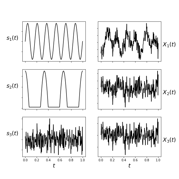
The individual signals ($s_i(t)$) and their mixtures ($X_i(t)$) are
shown in Figure. To recover the individual signals using ICA,
we use the FastICA object and fit the parameters on the X matrix,
from sklearn.decomposition import FastICA
ica = FastICA()
# estimate unknown S matrix
S_=ica.fit_transform(X)
The results of this estimation are shown in Figure, showing that ICA is able to recover the original signals from the observed mixture. Note that ICA is unable to distinguish the signs of the recovered signals or preserve the order of the input signals.
fig,axs=subplots(3,2,sharex=True)
fig.set_size_inches((8,8))
X = np.array(X)

_=axs[0,1].plot(t,-S_[:,2],'k-')
_=axs[1,1].plot(t,-S_[:,1],'k-')
_=axs[2,1].plot(t,-S_[:,0],'k-')
_=axs[0,0].plot(t,s1,'k-')
_=axs[1,0].plot(t,s2,'k-')
_=axs[2,0].plot(t,s3,'k-')

_=axs[2,0].set_xlabel('$t$',fontsize=18)
_=axs[2,1].set_xlabel('$t$',fontsize=18)
_=axs[0,0].set_ylabel('$s_1(t)$        ',fontsize=18,rotation='horizontal')
_=axs[1,0].set_ylabel('$s_2(t)$        ',fontsize=18,rotation='horizontal')
_=axs[2,0].set_ylabel('$s_3(t)$        ',fontsize=18,rotation='horizontal')
for ax in axs.flatten():
    _=ax.yaxis.set_ticklabels('')

_=axs[0,1].set_ylabel('        $s_1^\prime(t)$',fontsize=18,rotation='horizontal')
_=axs[1,1].set_ylabel('        $s_2^\prime(t)$',fontsize=18,rotation='horizontal')
_=axs[2,1].set_ylabel('        $s_3^\prime(t)$',fontsize=18,rotation='horizontal')
_=axs[0,1].yaxis.set_label_position("right")
_=axs[1,1].yaxis.set_label_position("right")
_=axs[2,1].yaxis.set_label_position("right")

fig.savefig('fig-machine_learning/pca_009.png')
The left column shows the original signals and the right column shows the signals that ICA was able to recover. They match exactly, outside of a possible sign change.
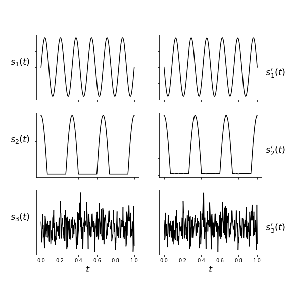
To develop some intuition as to how ICA accomplishes this feat, consider the following two-dimensional situation with two uniformly distributed independent variables, $u_x,u_y \sim \mathcal{U}[0,1]$. Suppose we apply the following orthogonal rotation matrix to these variables,
The left panel shows two classes labeled on the $u_x,u_y$ uniformly independent random variables. The right panel shows these random variables after a rotation, which removes their mutual independence and makes it hard to separate the two classes along the coordinate directions.
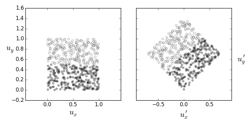
The so-rotated variables $u_x^\prime,u_y^\prime$ are no longer independent, as shown in Figure. Thus, one way to think about ICA is as a search through orthogonal matrices so that the independence is restored. This is where the prohibition against Gaussian distributions arises. The two dimensional Gaussian distribution of independent variables is proportional the following,
Now, if we similarly rotated the $\mathbf{x}$ vector as,
the resulting density for $\mathbf{y}$ is obtained by plugging in the following,
because the inverse of an orthogonal matrix is its transpose, we obtain
In other words, the transformation is lost on the $\mathbf{y}$ variable. This means that ICA cannot search over orthogonal transformations if it is blind to them, which explains the restriction of Gaussian random variables. Thus, ICA is a method that seeks to maximize the non-Gaussian-ness of the transformed random variables. There are many methods to doing this, some of which involve cumulants and others that use the negentropy,
where $\mathcal{H}(Z)$ is the information entropy of the Gaussian random variable $Z$ that has the same variance as $Y$. Further details would take us beyond our scope, but that is the outline of how the FastICA algorithm works.
The implementation of this method in Scikit-learn includes two different ways of extracting more than one independent source component. The deflation method iteratively extracts one component at a time using a incremental normalization step. The parallel method also uses the single-component method but carries out normalization of all the components simultaneously, instead of for just the newly computed component. Because ICA extracts independent components, a whitening step is used beforehand to balance the correlated components from the data matrix. Whereas PCA returns uncorrelated components along dimensions optimal for Gaussian random variables, ICA returns components that are as far from the Gaussian density as possible.
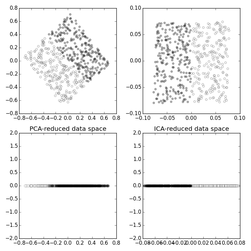
The left panel on Figure shows the orignal uniform random sources. The white and black colors distinguish between two classes. The right panel shows the mixture of these sources, which is what we observe as input features. The top row of Figure shows the PCA (left) and ICA (right) transformed data spaces. Notice that ICA is able to un-mix the two random sources whereas PCA transforms along the dominant diagonal. Because ICA is able to preserve the class membership, the data space can be reduced to two non-overlapping sections, as shown. However, PCA cannot achieve a similiar separation because the classes are mixed along the dominant diagonal that PCA favors as the main component in the decomposition.
The panel on the top left shows two classes in a plane after a rotation. The bottom left panel shows the result of dimensionality reduction using PCA, which causes mixing between the two classes. The top right panel shows the ICA transformed output and the lower right panel shows that, because ICA was able to un-rotate the data, the lower dimensional data maintains the separation between the classes.
For a good principal component analysis treatment, see [richert2013building], [alpaydin2014introduction], [cuesta2013practical], and [izenman2008modern]. Independent Component Analysis is discussed in more detail in [hyvarinen2004independent].