from IPython.display import Image
Image('../../Python_probability_statistics_machine_learning_2E.png',width=200)
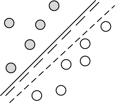
Support Vector Machines (SVM) originated from the statistical learning theory developed by Vapnik-Chervonenkis. As such, it represents a deep application of statistical theory that incorporates the VC dimension concepts we discussed in the first section. Let's start by looking at some pictures. Consider the two-dimensional classification problem shown in Figure. Figure shows two classes (gray and white circles) that can be separated by any of the lines shown. Specifically, any such separating line can be written as the locus of points ($\mathbf{x}$) in the two-dimensional plane that satisfy the following,
In the two-dimensional plane, the two classes (gray and white circles) are easily separated by any one of the lines shown.

To classify an arbitrary $\mathbf{x}$ using this line, we just compute the sign of $\beta_0+\boldsymbol{\beta}^T \mathbf{x}$ and assign one class to the positive sign and the other class to the negative sign. To uniquely specify such a separating line (or, hyperplane in a higher-dimensional space) we need additional criteria.
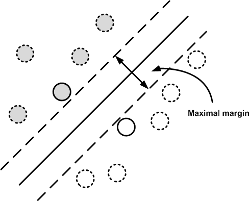
Figure shows the data with two bordering parallel lines that form a margin around the central separating line. The maximal margin algorithm finds the widest margin and the unique separating line. As a consequence, the algorithm uncovers the elements in the data that touch the margins. These are the support elements. The other elements away from the border are not relevant to the solution. This reduces model variance because the solution is insensitive to the removal of elements other than these supporting elements (usually a small minority).
The maximal margin algorithm finds the separating line that maximizes the margin shown. The elements that touch the margins are the support elements. The dotted elements are not relevant to the solution.

To see how this works for linearly separable classes, consider a training set consisting of $\lbrace (\mathbf{x},y) \rbrace$ where $y\in \lbrace -1,1 \rbrace$. For any point $\mathbf{x}_i$, we compute the functional margin as $\hat{ \gamma_i }=y_i (\beta_0 + \boldsymbol{\beta}^T \mathbf{x}_i)$. Thus, $\hat{\gamma}_i >0$ when $\mathbf{x}_i$ is correctly classified. The geometrical margin is $\gamma = \hat{\gamma}/\lVert\boldsymbol{\beta}\rVert$. When $\mathbf{x}_i$ is correctly classified, the geometrical margin is equal to the perpendicular distance from $\mathbf{x}_i$ to the line. Let's look see how the maximal margin algorithm works.
Let $M$ be the width of the margin. The maximal margin algorithm is can be formulated as a quadratic programming problem. We want to simultaneously maximize the margin $M$ while ensuring that all of the data points are correctly classified.
The first line says we want to generate a maximum value for $M$ by adjusting $\beta_0$ and $\boldsymbol{\beta}$ while keeping $\lVert\boldsymbol{\beta}\rVert=1$. The functional margins for each $i^{th}$ data element are the constraints to the problem and must be satisfied for every proposed solution. In words, the constraints enforce that the elements have to be correctly classified and outside of the margin around the separating line. With some reformulation, it turns out that $M=1/\lVert\boldsymbol{\beta}\rVert$ and this can be put into the following standard format,
This is a convex optimization problem and can be solved using powerful methods in that area.
The situation becomes more complex when the two classes are not separable and we have to allow some unavoidable mixing between the two classes in the solution. This means that the contraints have to modified as in the following,
where the $\xi_i$ are the slack variables and represent the proportional amount tha the prediction is on the wrong side of the margin. Thus, elements are misclassified when $\xi_i>1$. With these additional variables, we have a more general formulation of the convex optimization problem,
which can be rewritten in the following equivalent form,
Because the $\xi_i$ terms are all positive, the objective is to maximize the margin (i.e., minimize $\lVert\boldsymbol{\beta}\rVert$) while minimizing the proportional drift of the predictions to the wrong side of the margin (i.e., $C \sum \xi_i$). Thus, large values of $C$ shunt algorithmic focus towards the correctly classified points near the decision boundary and small values focus on further data. The value $C$ is a hyperparameter for the SVM.
The good news is that all of these complicated pieces are handled neatly inside of Scikit-learn. The following sets up the linear kernel for the SVM (more on kernels soon),
from sklearn.datasets import make_blobs
from sklearn.svm import SVC
sv = SVC(kernel='linear')
We can create some synthetic data using make_blobs and then
fit it to the SVM,
X,y=make_blobs(n_samples=200, centers=2, n_features=2,
               random_state=0,cluster_std=.5)
sv.fit(X,y)
After fitting, the SVM now has the estimated support vectors and the
coefficients of the $\boldsymbol{\beta}$ in the sv.support_vectors_ and
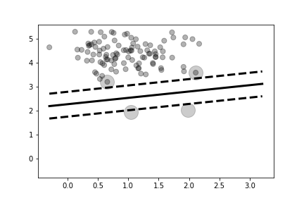
sv.coef_ attributes, respectively. Figure shows the two
sample classes (white and gray circles) and the line separating them that was
found by the maximal margin algorithm. The two parallel dotted lines show the
margin. The large circles enclose the support vectors, which are the data
elements that are relevant to the solution. Notice that only these elements
can touch the edges of the margins.
%matplotlib inline

from matplotlib.pylab import subplots
import numpy as np
xi = np.linspace(X[:,0].min(),X[:,0].max(),100)

fig,ax=subplots()
_=ax.scatter(X[:,0],X[:,1],c=y,s=50,cmap='gray',marker='o',alpha=.3)
_=ax.plot(sv.support_vectors_[:,0],sv.support_vectors_[:,1],'ko',markersize=20,alpha=.2)
_=ax.plot(xi,-sv.coef_[0,0]/sv.coef_[0,1]*xi- sv.intercept_/sv.coef_[0,1],'k',lw=3.)
margin = np.linalg.norm(sv.coef_)
_=ax.plot(xi,-sv.coef_[0,0]/sv.coef_[0,1]*xi-(sv.intercept_+margin/2.)/sv.coef_[0,1],'--k',lw=3.)
_=ax.plot(xi,-sv.coef_[0,0]/sv.coef_[0,1]*xi-(sv.intercept_-margin/2.)/sv.coef_[0,1],'--k',lw=3.)
fig.savefig('fig-machine_learning/svm_003.png')
The two class shown (white and gray circles) are linearly separable. The maximal margin solution is shown by the dark black line in the middle. The dotted lines show the extent of the margin. The large circles indicate the support vectors for the maximal margin solution.

def draw_margins(sv,X,y,ax=None):
    sv.fit(X,y)
    xi = np.linspace(X[:,0].min(),X[:,0].max(),100)
    if ax is None: fig,ax=subplots()
    _=ax.scatter(X[:,0],X[:,1],c=y,s=50,cmap='gray',marker='o',alpha=.3)
    _=ax.plot(sv.support_vectors_[:,0],sv.support_vectors_[:,1],'ko',markersize=20,alpha=.2)
    _=ax.plot(xi,-sv.coef_[0,0]/sv.coef_[0,1]*xi- sv.intercept_/sv.coef_[0,1],'k',lw=3.)
    margin = np.linalg.norm(sv.coef_)
    _=ax.plot(xi,-sv.coef_[0,0]/sv.coef_[0,1]*xi- (sv.intercept_+margin/2.)/sv.coef_[0,1],'--k',lw=3.)
    _=ax.plot(xi,-sv.coef_[0,0]/sv.coef_[0,1]*xi- (sv.intercept_-margin/2.)/sv.coef_[0,1],'--k',lw=3.)
X, y = make_blobs(n_samples=50, centers=2, n_features=2,
                  cluster_std=1,random_state=0)

fig,axs = subplots(2,2,sharex=True,sharey=True)
#fig.set_size_inches((12,6))
sv = SVC(kernel='linear',C=.0100)
draw_margins(sv,X,y,ax=axs[0,0])
_=axs[0,0].set_title('C=0.01')
sv = SVC(kernel='linear',C=1)
draw_margins(sv,X,y,ax=axs[0,1])
_=axs[0,1].set_title('C=1')
sv = SVC(kernel='linear',C=100)
draw_margins(sv,X,y,ax=axs[1,0])
_=axs[1,0].set_title('C=100')
sv = SVC(kernel='linear',C=10000)
draw_margins(sv,X,y,ax=axs[1,1])
_=axs[1,1].set_title('C=10000')
fig.savefig('fig-machine_learning/svm_004.png')
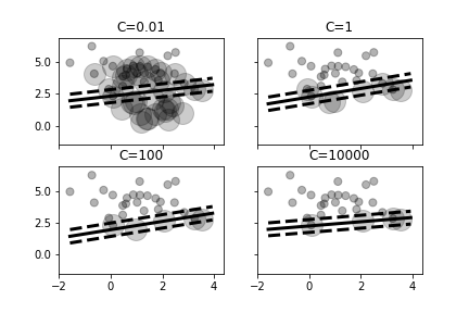
Figure shows what happens when the value of $C$ changes. Increasing this value emphasizes the $\xi$ part of the objective function in Equation 1. As shown in the top left panel, a small value for $C$ means that the algorithm is willing to accept many support vectors at the expense of maximizing the margin. That is, the proportional amount that predictions are on the wrong side of the margin is more acceptable with smaller $C$. As the value of $C$ increases, there are fewer support vectors because the optimization process prefers to eliminate support vectors that are far away from the margins and accept fewer of these that encroach into the margin. Note that as the value of $C$ progresses through this figure, the separating line tilts slightly.
The maximal margin algorithm finds the separating line that maximizes the margin shown. The elements that touch the margins are the support elements. The dotted elements are not relevant to the solution.

Kernel Tricks
Support Vector Machines provide a powerful method to deal with linear separations, but they can also apply to non-linear boundaries by exploiting the so-called kernel trick. The convex optimization formulation of the SVM includes a dual formulation that leads to a solution that requires only the inner-products of the features. The kernel trick is to substitute inner-products by nonlinear kernel functions. This can be thought of as mapping the original features onto a possibly infinite dimensional space of new features. That is, if the data are not linearly separable in two-dimensional space (for example) maybe they are separable in three-dimensional space (or higher)?
To make this concrete, suppose the original input space is $\mathbb{R}^n$ and we want to use a non-linear mapping $\psi:\mathbf{x} \mapsto \mathcal{F}$ where $\mathcal{F}$ is an inner-product space of higher dimension. The kernel trick is to calculate the inner-product in $\mathcal{F}$ using a kernel function, $K(\mathbf{x}_i,\mathbf{x}_j) = \langle \psi(\mathbf{x}_i),\psi(\mathbf{x}_j)\rangle$. The long way to compute this is to first compute $\psi(\mathbf{x})$ and then do the inner-product. The kernel-trick way to do it is to use the kernel function and avoid computing $\psi$. In other words, the kernel function returns what the inner-product in $\mathcal{F}$ would have returned if $\psi$ had been applied. For example, to achieve an $n^{th}$ polynomial mapping of the input space, we can use $\kappa(\mathbf{x}_i,\mathbf{x}_j)=(\mathbf{x}_i^T\mathbf{x}_j+\theta)^n$. For example, suppose the input space is $\mathbb{R}^2$ and $\mathcal{F}=\mathbb{R}^4$ and we have the following mapping,
The inner product in $\mathcal{F}$ is then,
In other words, the kernel is the square of the inner product in input space. The advantage of using the kernel instead of simply enlarging the feature space is computational because you only need to compute the kernel on all distinct pairs of the input space. The following example should help make this concrete. First we create some Sympy variables,
import sympy as S
x0,x1=S.symbols('x:2',real=True)
y0,y1=S.symbols('y:2',real=True)
Next, we create the $\psi$ function that maps into $\mathbb{R}^4$ and the corresponding kernel function,
psi = lambda x,y: (x**2,y**2,x*y,x*y)
kern = lambda x,y: S.Matrix(x).dot(y)**2
Notice that the inner product in $\mathbb{R}^4$ is equal to the kernel function, which only uses wthe $\mathbb{R}^2$ variables.
print(S.Matrix(psi(x0,x1)).dot(psi(y0,y1)))
print(S.expand(kern((x0,x1),(y0,y1)))) # same as above
Polynomial Regression Using Kernels. Recall our favorite linear regression problem from the regularization chapter,
where $\mathbf{X}$ is a $n\times m$ matrix with $m>n$. As we discussed, there are multiple solutions to this problem. The least-squares solution is the following:
Given a new feature vector $\mathbf{x}$, the corresponding estimator for $\mathbf{y}$ is the following,
Using the kernel trick, the solution can be written more generally as the following,
where the $n\times n$ kernel matrix $\mathbf{K}$ replaces $\mathbf{X}\mathbf{X}^T$ and where $\mathbf{k}(\mathbf{x})$ is a $n$-vector of components $\mathbf{k}(\mathbf{x})=[\kappa(\mathbf{x}_i,\mathbf{x})]$ and where $\mathbf{K}_{i,j}=\kappa(\mathbf{x}_i,\mathbf{x}_j)$ for the kernel function $\kappa$. With this more general setup, we can substitute $\kappa(\mathbf{x}_i,\mathbf{x}_j)=(\mathbf{x}_i^T\mathbf{x}_j+\theta)^n$ for $n^{th}$-order polynomial regression [bauckhagenumpy]. Note that ridge regression can also be incorporated by inverting $(\mathbf{K}+\alpha \mathbf{I})$, which can help stabilize poorly conditioned $\mathbf{K}$ matrices with a tunable $\alpha$ hyper-parameter [bauckhagenumpy].
For some kernels, the enlarged $\mathcal{F}$ space is infinite-dimensional. Mercer's conditions provide technical restrictions on the kernel functions. Powerful and well-studied kernels have been implemented in Scikit-learn. The advantage of kernel functions may evaporate for when $n\rightarrow m$ in which case using the $\psi$ functions instead can be more practicable.
from matplotlib.pylab import cm
xi = np.linspace(X[:,0].min(),X[:,0].max(),100)
yi = np.linspace(X[:,1].min(),X[:,1].max(),100)

fig,ax=subplots()
_=ax.scatter(X[:,0],X[:,1],c=y,s=50,cmap='gray',marker='o',alpha=.3)
Xi,Yi = np.meshgrid(xi,yi)
Zi=sv.predict(np.c_[Xi.ravel(),Yi.ravel()]).reshape(Xi.shape)

_=ax.contourf(Xi,Yi,Zi,cmap=cm.Paired,alpha=0.2);
fig.savefig('fig-machine_learning/svm_005.png')