from IPython.display import Image
Image('../../Python_probability_statistics_machine_learning_2E.png',width=200)

Useful Inequalities

In practice, few quantities can be analytically calculated. Some knowledge of bounding inequalities helps find the ballpark for potential solutions. This sections discusses three key inequalities that are important for probability, statistics, and machine learning.

Markov's

Inequality

Let $X$ be a non-negative random variable and suppose that $\mathbb{E}(X) < \infty$. Then, for any $t>0$,

$$ \mathbb{P}(X>t)\leq \frac{\mathbb{E}(X)}{t} $$

This is a foundational inequality that is used as a stepping stone to other inequalities. It is easy to prove. Because $X>0$, we have the following,

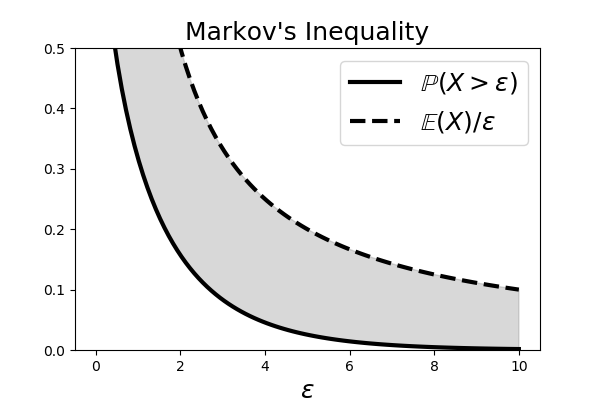
$$ \begin{align*} \mathbb{E}(X)&=\int_0^\infty x f_x(x)dx =\underbrace{\int_0^t x f_x(x)dx}_{\text{omit this}}+\int_t^\infty x f_x(x)dx \\\ &\ge\int_t^\infty x f_x(x)dx \ge t\int_t^\infty f_x(x)dx = t \mathbb{P}(X>t) \end{align*} $$

The step that establishes the inequality is the part where the $\int_0^t x f_x(x)dx$ is omitted. For a particular $f_x(x)$ that may be concentrated around the $[0,t]$ interval, this could be a lot to throw out. For that reason, the Markov Inequality is considered a loose inequality, meaning that there is a substantial gap between both sides of the inequality. For example, as shown in Figure, the $\chi^2$ distribution has a lot of its mass on the left, which would be omitted in the Markov Inequality. Figure shows the two curves established by the Markov Inequality. The gray shaded region is the gap between the two terms and indicates that looseness of the bound (fatter shaded region) for this case.

The $\chi_1^2$ density has much of its weight on the left, which is excluded in the establishment of the Markov Inequality.

The shaded area shows the region between the curves on either side of the Markov Inequality.

Chebyshev's Inequality

Chebyshev's Inequality drops out directly from the Markov Inequality. Let $\mu=\mathbb{E}(X)$ and $\sigma^2=\mathbb{V}(X)$. Then, we have

$$ \mathbb{P}(\vert X-\mu\vert \ge t) \le \frac{\sigma^2}{t^2} $$

Note that if we normalize so that $Z=(X-\mu)/\sigma$, we have $\mathbb{P}(\vert Z\vert \ge k) \le 1/k^2$. In particular, $\mathbb{P}(\vert Z\vert \ge 2) \le 1/4$. We can illustrate this inequality using Sympy statistics module,

import sympy
import sympy.stats as ss
t=sympy.symbols('t',real=True)
x=ss.ChiSquared('x',1)

To get the left side of the Chebyshev inequality, we have to write this out as the following conditional probability,

r = ss.P((x-1) > t,x>1)+ss.P(-(x-1) > t,x<1)

We could take the above expression, which is a function of $t$ and attempt to compute the integral, but that would take a very long time (the expression is very long and complicated, which is why we did not print it out above). In this situation, it's better to use the built-in cumulative density function as in the following (after some rearrangement of the terms),

w=(1-ss.cdf(x)(t+1))+ss.cdf(x)(1-t)

To plot this, we can evaluated at a variety of t values by using the .subs substitution method, but it is more convenient to use the lambdify method to convert the expression to a function.

fw=sympy.lambdify(t,w)

Then, we can evaluate this function using something like

[fw(i) for i in [0,1,2,3,4,5]]

[1.0,
 0.157299207050285,
 (0.08326451666355039+0j),
 (0.04550026389635842+0j),
 (0.0253473186774682+0j),
 (0.014305878435429631+0j)]

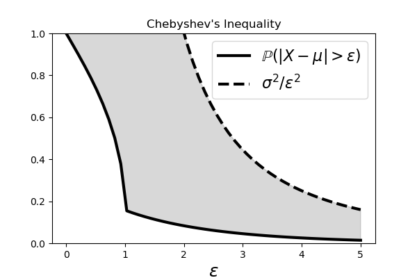
to produce the following Figure.

The shaded area shows the region between the curves on either side of the Chebyshev Inequality.

Programming Tip.

Note that we cannot use vectorized inputs for the lambdify function because it contains embedded functions that are only available in Sympy. Otherwise, we could have used lambdify(t,fw,numpy) to specify the corresponding functions in Numpy to use for the expression.

Hoeffding's Inequality

Hoeffding's Inequality is similar, but less loose, than Markov's Inequality. Let $X_1,\ldots,X_n$ be iid observations such that $\mathbb{E}(X_i)=\mu$ and $a\le X_i \le b$. Then, for any $\epsilon>0$, we have

$$ \mathbb{P}(\vert \overline{X}_n -\mu\vert \ge \epsilon) \le 2 \exp(-2 n\epsilon^2/(b-a)^2) $$

where $\overline{X}_n = \tfrac{1}{n}\sum_i^n X_i$. Note that we further assume that the individual random variables are bounded.

Corollary. If $X_1,\ldots,X_n$ are independent with $\mathbb{P}(a\le X_i\le b)=1$ and all with $\mathbb{E}(X_i)=\mu$. Then, we have

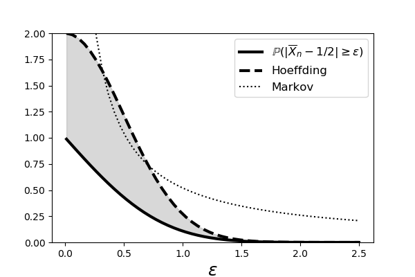
$$ \vert\overline{X}_n-\mu\vert \le \sqrt{\frac{c}{2 n}\log \frac{2}{\delta}} $$

where $c=(b-a)^2$. We will see this inequality again in the machine learning chapter. Figure shows the Markov and Hoeffding bounds for the case of ten identically and uniformly distributed random variables, $X_i \sim \mathcal{U}[0,1]$. The solid line shows $\mathbb{P}(\vert \overline{X}_n - 1/2 \vert > \epsilon)$. Note that the Hoeffding Inequality is tighter than the Markov Inequality and that both of them merge when $\epsilon$ gets big enough.

This shows the Markov and Hoeffding bounds for the case of ten identically and uniformly distributed random variables.

Proof of Hoeffding's Inequality

We will need the following lemma to prove Hoeffding's inequality.

Lemma Let $X$ be a random variable with $\mathbb{E}(X)=0$ and $a\le X\le b$. Then, for any $s>0$, we have the following,

$$ \begin{equation} \mathbb{E}(e^{s X}) \le e^{s^2(b-a)^2/8} \label{_auto1} \tag{1} \end{equation} $$

Because $X$ is contained in the closed interval $[a,b]$, we can write it as a convex combination of the endpoints of the interval.

$$ X = \alpha_1 a + \alpha_2 b $$

where $\alpha_1+\alpha_2=1$. Solving for the $\alpha_i$ terms, we have

$$ \begin{align*} \alpha_1 = & \frac{x-a}{b-a} \\ \alpha_2 = & \frac{b-x}{b-a} \end{align*} $$

From Jensen's inequality, for a convex functions $f$, we know that

$$ f\left(\sum \alpha_i x_i\right) \le \sum \alpha_i f(x_i) $$

Given the convexity of $e^X$, we therefore have,

$$ e^{s X} \le \alpha_1 e^{s a} + \alpha_2 e^ {s b} $$

With $\mathbb{E}(X)=0$, we can write the expectation of both sides

$$ \mathbb{E}(e^{s X}) \le \mathbb{E}(\alpha_1) e^{s a} +\mathbb{E}(\alpha_2) e^{s b} $$

with $\mathbb{E}(\alpha_1)=\frac{b}{b-a}$ and $\mathbb{E}(\alpha_2)=\frac{-a}{b-a}$. Thus, we have

$$ \mathbb{E}(e^{s X}) \le \frac{b}{b-a} e^{s a} -\frac{a}{b-a} e^{s b} $$

Using $p:=\frac{-a}{b-a}$, we can rewrite the following,

$$ \frac{b}{b-a} e^{s a} -\frac{a}{b-a} e^{s b} = (1-p)e^{s a} + p e^{s b} =: e^{\phi(u)} $$

where

$$ \phi(u)=-p u + \log(1-p+p e^{u}) $$

and $u=s(b-a)$. Note that $\phi(0)=\phi'(0)=0$. Also, $\phi''(0) = p(1-p)\le 1/4$. Thus, the Taylor expansion of $\phi(u)\approx \frac{u^2}{2}\phi''(t) \le \frac{u^2}{8}$ for $t\in [0,u] \blacksquare$.

To prove Hoeffding's inequality, we start with Markov's inequality,

$$ \mathbb{P}(X\ge\epsilon)\le \frac{\mathbb{E}(X)}{\epsilon} $$

Then, given $s>0$, we have the following,

$$ \mathbb{P}(X\ge\epsilon)=\mathbb{P}(e^{s X} \ge e^{s\epsilon}) \le \frac{\mathbb{E}(e^{s X})}{e^{s \epsilon}} $$

We can write the one-sided Hoeffding inequality as the following,

$$ \begin{align*} \mathbb{P}(\overline{X}_n -\mu\ge\epsilon) & \le e^{-s\epsilon}\mathbb{E}(\exp(\frac{s}{n}\sum_{i=1}^n (X_i-\mathbb{E}(X_i)))) \\ & = e^{-s\epsilon}\prod_{i=1}^n\mathbb{E}(e^{ \frac{s}{n} (X_i-\mathbb{E}(X_i)) }) \\ & \le e^{-s\epsilon}\prod_{i=1}^n e^{\frac{s^2}{n^2}(b-a)^2/8 } \\ & = e^{-s\epsilon} e^{\frac{s^2}{n}(b-a)^2/8} \end{align*} $$

Now, we want to pick $s>0$ to minimize this upper bound. Then, with $s=\frac{4 n\epsilon}{(b-a)^2}$

$$ \mathbb{P}(\overline{X}_n-\mu\ge\epsilon)\le e^{-\frac{2 n\epsilon^2}{(b-a)^2}} $$

The other side of the inequality follows similarly to obtain Hoeffding's inequality $\blacksquare$.

Jensen's Inequality

If $f$ is a convex function with random variable $v$, then

$$ \mathbb{E}(f(v))\ge f(\mathbb{E}(v)) $$

The proof of this is straightforward. Define $L(v) = a v +b $ with $a,b\in \mathbb{R}$. Choose $a$ and $b$ so that $L(\mathbb{E}(v))=f(\mathbb{E}(v))$ which makes $L$ tangent to $f$ at $\mathbb{E}(v)$. By the convexity of $f$, we have $f(v)\ge L(v)$. We can take the expectation of both sides of this,

$$ \begin{align*} \mathbb{E}(f(v)) \ge & \mathbb{E}(L(v)) \\ = & \mathbb{E}(a v+b) \\ = & a\mathbb{E}(v)+b \\ = & L(\mathbb{E}(v)) \\ = & f(\mathbb{E}(v)) \end{align*} $$

equality holds when $f$ is linear. For a concave function $f$, the sense of the inequality is reversed.